Higher-Order MuP: A More Concise Yet Profound Spectral Condition Scaling

In the article "A Preliminary Exploration of MuP: Cross-Model Scaling Laws for Hyperparameters", we derived MuP (Maximal Update Parametrization) based on scale invariance in forward propagation, backward propagation, loss increment, and feature variation. For some readers, this process might still seem somewhat cumbersome, although it is significantly simplified compared to the original paper. It's worth noting that we introduced MuP relatively comprehensively within a single article, while the MuP paper is actually the fifth in the author's Tensor Programs series!

Preparatory Work#

As the name suggests, the spectral condition is related to the spectral norm. Its starting point is a fundamental inequality of the spectral norm:

where $\boldsymbol{x}\in\mathbb{R}^{d_{in}}, \boldsymbol{W}\in\mathbb{R}^{d_{in}\times d_{out}}$, and as for $\Vert\cdot\Vert_2$, we can call it the "$2$-norm". For $\boldsymbol{x},\boldsymbol{x}\boldsymbol{W}$, they are both vectors, so the $2$-norm is the vector length; while $\boldsymbol{W}$ is a matrix, and its $2$-norm is also called the spectral norm, which equals the smallest constant $C$ such that $\Vert\boldsymbol{x}\boldsymbol{W}\Vert_2\leq C\Vert\boldsymbol{x}\Vert_2$ holds for all $\boldsymbol{x}$. In other words, the above inequality is a direct consequence of the definition of spectral norm and requires no additional proof.

Regarding spectral norm, readers can also refer to blog posts such as "Lipschitz Constraints in Deep Learning: Generalization and Generative Models", "The Path of Low-Rank Approximation (II): SVD", etc. We won't expand on it here. A matrix also has a simpler $F$-norm, which is a straightforward extension of vector length:

From the perspective of singular values, the spectral norm equals the largest singular value of the matrix, while the $F$-norm equals the square root of the sum of squares of all singular values. Similarly, we can also define the "Nuclear Norm", which equals the sum of all singular values:

Matrix norms such as spectral norm, $F$-norm, and nuclear norm that can be expressed through singular values all belong to one type of Schatten-p norms. Finally, let's define RMS (Root Mean Square), which is a variant of vector length:

If we extend this to matrices, then $\Vert\boldsymbol{W}\Vert_{RMS} = \Vert \boldsymbol{W}\Vert_F/\sqrt{d_{in} d_{out}}$. Actually, it's easy to understand from the name: vector length or matrix $F$-norm can be called "Root Sum Square", while RMS replaces Sum with Mean, mainly serving as an average scale indicator for vector or matrix elements. Now substituting RMS into inequality (1), we obtain:

Desired Properties#

Our previous approach to deriving MuP involved carefully analyzing the forms of forward propagation, backward propagation, loss increment, and feature variation, and adjusting initialization and learning rates to achieve their scale invariance. The spectral condition "refines and simplifies" this by finding that focusing only on forward propagation and feature variation is sufficient.

1. $\Vert\boldsymbol{x}_k\Vert_{RMS}=\mathcal{\Theta}(1)$ is easy to understand—it represents the stability of forward propagation, which was also included in the derivation in the previous article.

2. $\Delta\boldsymbol{x}_k$ represents the change in $\boldsymbol{x}_k$ caused by parameter changes, so $\Vert\Delta\boldsymbol{x}_k\Vert_{RMS}=\mathcal{\Theta}(1)$ combines the requirements of backward propagation and feature variation.

The proof is not difficult. The key here is that we assume $\Vert\boldsymbol{x}_k\Vert_{RMS}=\mathcal{\Theta}(1)$ and $\Vert\Delta\boldsymbol{x}_k\Vert_{RMS}=\mathcal{\Theta}(1)$ hold for each layer, so the last layer naturally satisfies this as well. Assume the model has $K$ layers in total, with the single-sample loss function as $\ell$, which is a function of $\boldsymbol{x}_K$ i.e., $\ell(\boldsymbol{x}_K)$. For simplicity, we omit label inputs here since they are not variables for the following analysis.

Based on the assumption, $\Vert\boldsymbol{x}_K\Vert_{RMS}$ is $\mathcal{\Theta}(1)$, so naturally $\ell(\boldsymbol{x}_K)$ is $\mathcal{\Theta}(1)$; also since $\Vert\Delta\boldsymbol{x}_K\Vert_{RMS}$ is $\mathcal{\Theta}(1)$, we have $\Vert\boldsymbol{x}_K + \Delta\boldsymbol{x}_K\Vert_{RMS}\leq \Vert\boldsymbol{x}_K\Vert_{RMS} + \Vert\Delta\boldsymbol{x}_K\Vert_{RMS}$ which is also $\mathcal{\Theta}(1)$, thus $\ell(\boldsymbol{x}_K + \Delta\boldsymbol{x}_K)$ is $\mathcal{\Theta}(1)$, and therefore:

Thus, the single-sample loss increment $\Delta \ell$ is $\mathcal{\Theta}(1)$, and $\Delta\mathcal{L}$ is the average of all $\Delta \ell$, so it is also $\mathcal{\Theta}(1)$. This proves that $\Vert\boldsymbol{x}_k\Vert_{RMS}=\mathcal{\Theta}(1)$ and $\Vert\Delta\boldsymbol{x}_k\Vert_{RMS}=\mathcal{\Theta}(1)$ automatically include $\Delta\mathcal{L}=\mathcal{\Theta}(1)$. The principle is simply that $\Delta\mathcal{L}$ is a function of the last layer's output and its increment—once they are stable, $\Delta\mathcal{L}$ naturally becomes stable.

Spectral Condition#

Next, let's examine how to achieve the two desired properties. Since neural networks primarily consist of matrix multiplications, we first consider the simplest linear layer $\boldsymbol{x}_k = \boldsymbol{x}_{k-1} \boldsymbol{W}_k$, where $\boldsymbol{W}_k\in\mathbb{R}^{d_{k-1}\times d_k}$. To satisfy the condition $\Vert\boldsymbol{x}_k\Vert_{RMS}=\mathcal{\Theta}(1)$, the spectral condition does not assume independent identically distributed variables and calculate expectations and variances as in traditional initialization analysis, but directly applies inequality (5):

Note that this inequality can achieve equality, and in some sense is the most precise. So if the input $\Vert\boldsymbol{x}_{k-1}\Vert_{RMS}$ is already $\mathcal{\Theta}(1)$, then to make the output $\Vert\boldsymbol{x}_k\Vert_{RMS}=\mathcal{\Theta}(1)$, we need:

After analyzing $\Vert\boldsymbol{x}_k\Vert_{RMS}$, we come to $\Vert\Delta\boldsymbol{x}_k\Vert_{RMS}$. The source of increment $\Delta\boldsymbol{x}_k$ has two parts: first, parameters change from $\boldsymbol{W}_k$ to $\boldsymbol{W}_k+\Delta \boldsymbol{W}_k$; second, input $\boldsymbol{x}_{k-1}$ changes due to parameter variations from $\boldsymbol{x}_{k-1}$ to $\boldsymbol{x}_{k-1} + \Delta\boldsymbol{x}_{k-1}$, so:

Therefore:

Analyzing term by term:

From this, we can see that to achieve $\Vert\Delta\boldsymbol{x}_k\Vert_{RMS}=\mathcal{\Theta}(1)$, we need:

This is the second spectral condition—the requirement on the spectral norm of $\Delta\boldsymbol{W}_k$.

Spectral Normalization#

Now we have two spectral conditions (8) and (12). Next, we need to consider how to design the model and its optimization to satisfy these two conditions.

Note that both $\boldsymbol{W}_k$ and $\Delta \boldsymbol{W}_k$ are matrices. The standard method to make a matrix satisfy spectral norm conditions is usually spectral normalization (SN), and this case is no exception. First, we want the initialized $\boldsymbol{W}_k$ to satisfy $\Vert\boldsymbol{W}_k\Vert_2=\mathcal{\Theta}\left(\sqrt{\frac{d_k}{d_{k-1}}}\right)$. This can be achieved by selecting an arbitrary initialization matrix $\boldsymbol{W}_k'$ and then applying spectral normalization:

Here $\sigma > 0$ is a scale-independent constant. Similarly, for the update $\boldsymbol{\Phi}_k$ provided by any optimizer, we can reconstruct $\Delta \boldsymbol{W}_k$ through spectral normalization:

where $\eta > 0$ is also a scale-independent constant (learning rate), ensuring that each step satisfies $\Vert\Delta\boldsymbol{W}_k\Vert_2=\mathcal{\Theta}\left(\sqrt{\frac{d_k}{d_{k-1}}}\right)$. Since both initialization and each step update have spectral norms satisfying $\mathcal{\Theta}\left(\sqrt{\frac{d_k}{d_{k-1}}}\right)$, $\Vert\boldsymbol{W}_k\Vert_2$ also satisfies $\mathcal{\Theta}\left(\sqrt{\frac{d_k}{d_{k-1}}}\right)$ throughout, thus meeting both spectral conditions.

Singular Value Clipping#

To achieve the spectral norm condition, besides spectral normalization as a standard method, we can also consider singular value clipping (SVC). This section is supplemented by the author and does not appear in the original paper, but it can explain some interesting results.

From the perspective of singular values, spectral normalization scales the largest singular value to 1 and proportionally scales the remaining singular values. Singular value clipping is somewhat more lenient—it only sets singular values greater than 1 to 1, without altering those already less than or equal to 1:

In contrast, spectral normalization is $\mathop{\text{SN}}(\boldsymbol{W})=\boldsymbol{U}(\boldsymbol{\Lambda}/\max(\boldsymbol{\Lambda}))\boldsymbol{V}^{\top}$. Replacing spectral normalization with singular value clipping, we obtain:

The drawback of singular value clipping is that it only guarantees the clipped spectral norm equals 1 when at least one singular value is greater than or equal to 1. If not satisfied, we can consider multiplying by $\lambda > 0$ and then clipping, i.e., changing to $\mathop{\text{SVC}}(\lambda\boldsymbol{W})$. However, different scaling factors yield different results, yet it's not easy to determine a suitable scaling factor. Nevertheless, we can consider a limiting version:

Here $\mathop{\text{msign}}$ is the matrix sign function $\mathop{\text{msign}}$ used in Muon (refer to "Appreciating Muon Optimizer: The Essential Leap from Vectors to Matrices"). Replacing spectral normalization or singular value clipping with $\mathop{\text{msign}}$, we obtain:

This actually gives us a generalized Muon optimizer. Standard Muon applies $\mathop{\text{msign}}$ to momentum, while this allows us to apply $\mathop{\text{msign}}$ to updates from any existing optimizer. Coincidentally, someone on Twitter recently experimented with applying $\mathop{\text{msign}}$ to Adam updates (they called it "Mudamw", link), finding it performed slightly better than Muon, as shown below:

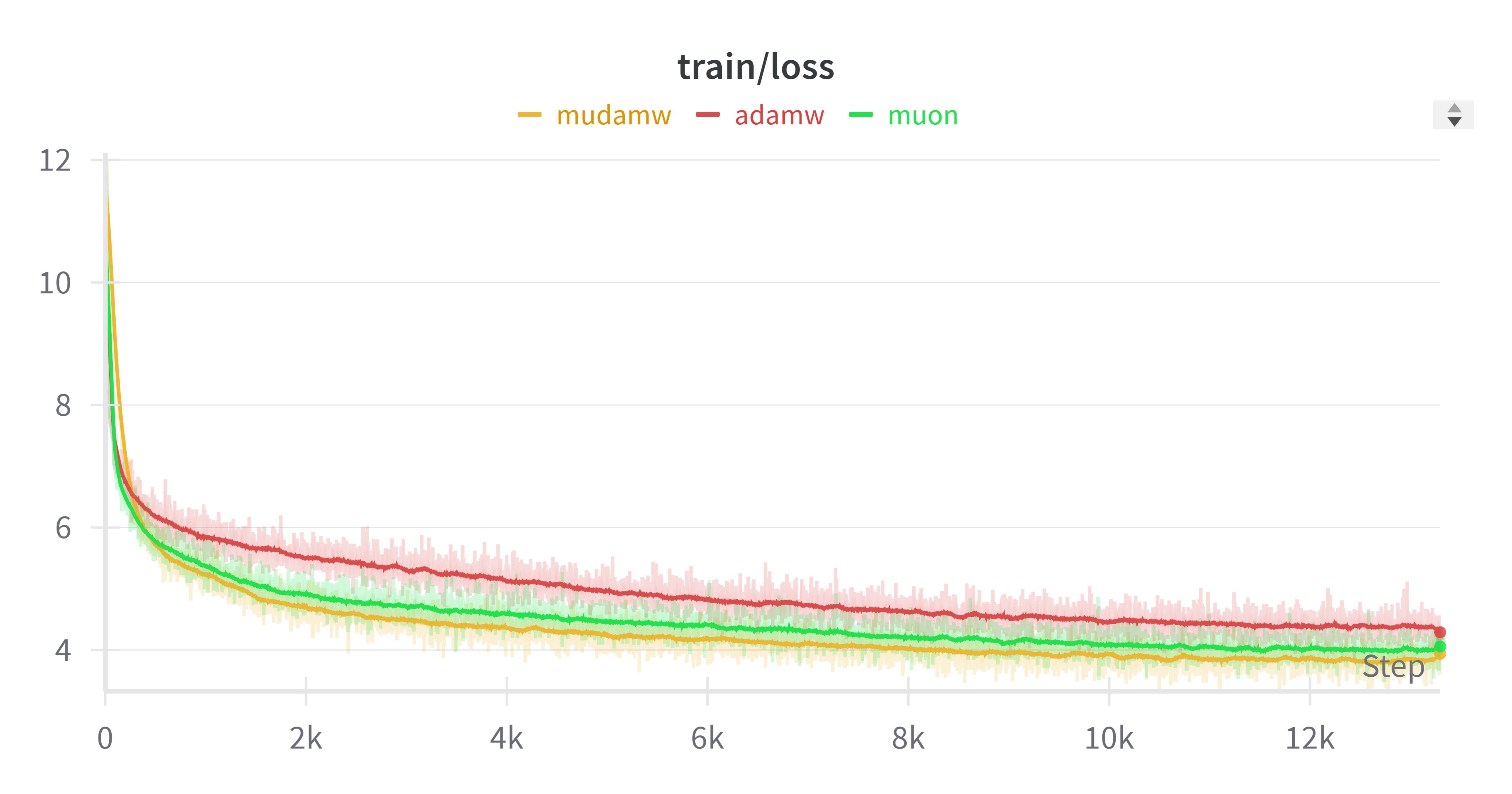
Adam+msign appears to outperform Muon (from Twitter @KyleLiang5)

Upon seeing this, we also tried it on small models and found we could reproduce similar conclusions! So perhaps applying $\mathop{\text{msign}}$ to existing optimizers might yield better results. The feasibility of this operation is difficult to explain within the original Muon framework, but here we interpret it as applying singular value clipping (or its limiting version) to updates, naturally leading to this result.

Approximation Estimation#

It's generally believed that operations related to SVD (Singular Value Decomposition), such as spectral normalization, singular value clipping, or $\mathop{\text{msign}}$, are relatively expensive. Therefore, we still hope to find simpler forms. Since our goal is only to find scaling laws between model scales, further simplification is indeed possible.

First, initialization. Initialization is a one-time operation, so even if computational cost is somewhat higher, it's not a big problem. Thus, the previous scheme of random initialization followed by spectral normalization/singular value clipping/$\mathop{\text{msign}}$ can still be retained. If we still want to refine further, we can utilize a statistical result: for a $d_{k-1}\times d_k$ matrix sampled independently from a standard normal distribution, its largest singular value is approximately $\sqrt{d_{k-1}} + \sqrt{d_k}$. This essentially means that as long as the sampling standard deviation is changed to:

it can meet the requirement $\Vert\boldsymbol{W}_k\Vert_2=\mathcal{\Theta}\left(\sqrt{\frac{d_k}{d_{k-1}}}\right)$ during initialization. As for the proof of this statistical result, readers can refer to materials such as "High-Dimensional Probability", "Marchenko-Pastur law", etc., which won't be expanded here.

Next, let's examine the update, which is relatively more troublesome because the spectral norm of an arbitrary update $\boldsymbol{\Phi}_k$ is not so easy to estimate. Here we need to utilize an empirical conclusion: gradient matrices of parameters are typically low-rank. This low-rank nature is not necessarily mathematically strict low-rank, but rather that the largest few (number independent of model scale) singular values significantly exceed the remaining singular values, making low-rank approximation feasible—this is also the theoretical foundation for various LoRA optimizations.

A direct corollary of this empirical assumption is the approximate equivalence between spectral norm and nuclear norm. Since spectral norm is the largest singular value and nuclear norm is the sum of all singular values, under the above assumption, the nuclear norm approximately equals the sum of the largest several singular values. Thus, the two are at least consistent in scale, i.e., $\mathcal{\Theta}(\Vert\nabla_{\boldsymbol{W}_k}\mathcal{L}\Vert_2)=\mathcal{\Theta}(\Vert\nabla_{\boldsymbol{W}_k}\mathcal{L}\Vert_*)$. Next, we utilize the relationship between $\Delta\mathcal{L}$ and $\Delta\boldsymbol{W}_k$:

Here $\langle\cdot,\cdot\rangle_F$ is the Frobenius inner product, i.e., flattening matrices into vectors and computing inner products. As for the inequality, it's due to a classical matrix inequality $\langle\boldsymbol{A},\boldsymbol{B}\rangle_F \leq \Vert\boldsymbol{A}\Vert_2\, \Vert\boldsymbol{B}\Vert_*$, similar to Holder's inequality. In fact, we proved precisely this when deriving Muon in "Appreciating Muon Optimizer: The Essential Leap from Vectors to Matrices". Based on the above and combined with the low-rank assumption of gradients, we have:

Don't forget that we have already proven earlier that satisfying the two spectral conditions necessarily implies $\Delta\mathcal{L}=\mathcal{\Theta}(1)$. Now combining with the above equation, we obtain that when $\Vert\Delta\boldsymbol{W}_k\Vert_2=\mathcal{\Theta}\left(\sqrt{\frac{d_k}{d_{k-1}}}\right)$, we have:

Learning Rate Strategy#

Applying estimate (22) to SGD, i.e., $\Delta \boldsymbol{W}_k = -\eta_k \nabla_{\boldsymbol{W}_k}\mathcal{L}$, according to equation (22) we have $\Vert\nabla_{\boldsymbol{W}_k}\mathcal{L}\Vert_2=\mathcal{\Theta}\left(\sqrt{\frac{d_{k-1}}{d_k}}\right)$. To achieve the goal $\Vert\Delta\boldsymbol{W}_k\Vert_2=\mathcal{\Theta}\left(\sqrt{\frac{d_k}{d_{k-1}}}\right)$, we need:

As for Adam, we still approximate with SignSGD $\Delta \boldsymbol{W}_k = -\eta_k \mathop{\text{sign}}(\nabla_{\boldsymbol{W}_k}\mathcal{L})$. Since $\mathop{\text{sign}}$ generally yields $\pm 1$, we have $\Vert\mathop{\text{sign}}(\nabla_{\boldsymbol{W}_k}\mathcal{L})\Vert_F = \mathcal{\Theta}(\sqrt{d_{k-1} d_k})$. Element-wise operations like $\mathop{\text{sign}}$ typically don't have special rank-increasing effects, so we believe $\mathop{\text{sign}}(\nabla_{\boldsymbol{W}_k}\mathcal{L})$ and $\nabla_{\boldsymbol{W}_k}\mathcal{L}$ are both low-rank. Thus, similar to nuclear norm, the $F$-norm and spectral norm will be of the same order, i.e., $\Vert\mathop{\text{sign}}(\nabla_{\boldsymbol{W}_k}\mathcal{L})\Vert_2 = \mathcal{\Theta}(\sqrt{d_{k-1} d_k})$.

Therefore, to achieve the goal $\Vert\Delta\boldsymbol{W}_k\Vert_2=\mathcal{\Theta}\left(\sqrt{\frac{d_k}{d_{k-1}}}\right)$, we need:

Regarding initialization, MuP has input variance $1/d_{in}$, output variance $1/d^2$, and remaining parameter variance $1/d$, while the spectral condition result has only one equation (19). But if we examine carefully, equation (19) already encompasses MuP's three cases: setting input, intermediate, and output matrix sizes as $d_{in}\times d,d\times d,d\times d_{out}$ respectively, substituting into equation (19) yields:

Some readers might wonder why we only consider $d\to\infty$. This is because $d_{in},d_{out}$ are task-related numbers, essentially constants. The variable model scale is only $d$, and MuP studies the asymptotic laws of hyperparameters with model scale, so it refers to the simplified laws when $d$ is sufficiently large.

Regarding learning rates, for SGD, MuP has input learning rate $d$, output learning rate $1/d$, and remaining parameter learning rate $1$. Note these relationships are proportional, not equal. The spectral condition result (23) similarly encompasses these three cases. Similarly, for Adam, MuP has input learning rate $1$, output learning rate $1/d$, and remaining parameter learning rate $1/d$. The spectral condition still describes these three cases with a single equation (24).

Article Summary#

This article introduces the upgraded version of MuP—the spectral condition. It starts from inequalities related to spectral norms to analyze conditions for stable model training, obtaining richer results than MuP in a more convenient way.