How Does Adam's Epsilon Affect Learning Rate Scaling Laws?

In the previous article "How Should Learning Rate Scale with Batch Size?", we discussed the scaling laws between learning rate and batch size from multiple perspectives. For the Adam optimizer, we employed the SignSGD approximation—a common technique for analyzing Adam. A natural question then arises: how scientific is it to approximate Adam using SignSGD?

We know that Adam's update denominator includes an $\epsilon$, originally intended to prevent division by zero, so its value is typically very close to zero, and we often choose to ignore it during theoretical analysis. However, in current LLM training, especially in low-precision training, we tend to choose relatively large $\epsilon$ values. This results in $\epsilon$ often exceeding the magnitude of gradient squares during the middle and later stages of training, making the presence of $\epsilon$ practically non-negligible.

Therefore, in this article, we attempt to explore how $\epsilon$ affects Adam's learning rate and batch size scaling laws, providing a reference computational scheme for related issues.

SoftSign#

Since this article follows the previous one, we won't repeat the background. To investigate the role of $\epsilon$, we switch from SignSGD to SoftSignSGD, i.e., from $\newcommand{sign}{\mathop{\text{sign}}}\tilde{\boldsymbol{\varphi}}_B = \sign(\tilde{\boldsymbol{g}}_B)$ to $\tilde{\boldsymbol{\varphi}}_B = \text{softsign}(\tilde{\boldsymbol{g}}_B)$, where:

This form undoubtedly aligns more closely with Adam. But before proceeding, we need to confirm whether $\epsilon$ is truly non-negligible to determine if further research is warranted.

It's worth noting that introducing $\epsilon$ actually provides an interpolation between Adam and SGD, because when $x\neq 0$:

Thus, the larger $\epsilon$ is, the more Adam's behavior approaches SGD.

Sigmoid Approximations#

Having confirmed the necessity of introducing $\epsilon$, we proceed with the analysis. During the analysis, we will repeatedly encounter sigmoid functions, so another preparatory step is to explore simple approximations for sigmoid functions.

Sigmoid functions are already familiar to most; the $\text{softsign}$ function introduced in the previous section is itself one example, the $\text{erf}$ function appearing in the previous article's analysis is another, along with $\tanh$, $\text{sigmoid}$, etc. Next, we handle sigmoid functions $S(x)$ satisfying the following characteristics:

1. Globally smooth and monotonically increasing;

2. Odd function, with range $[-1,1]$;

3. Slope at the origin is $k > 0$.

For such functions, we consider two approximations. The first is similar to $\text{softsign}$:

This is probably the simplest function preserving the three properties above for $S(x)$. The second approximation is based on the $\text{clip}$ function:

This is essentially a piecewise linear function, sacrificing global smoothness, but piecewise linearity makes integration easier, as we will see shortly.

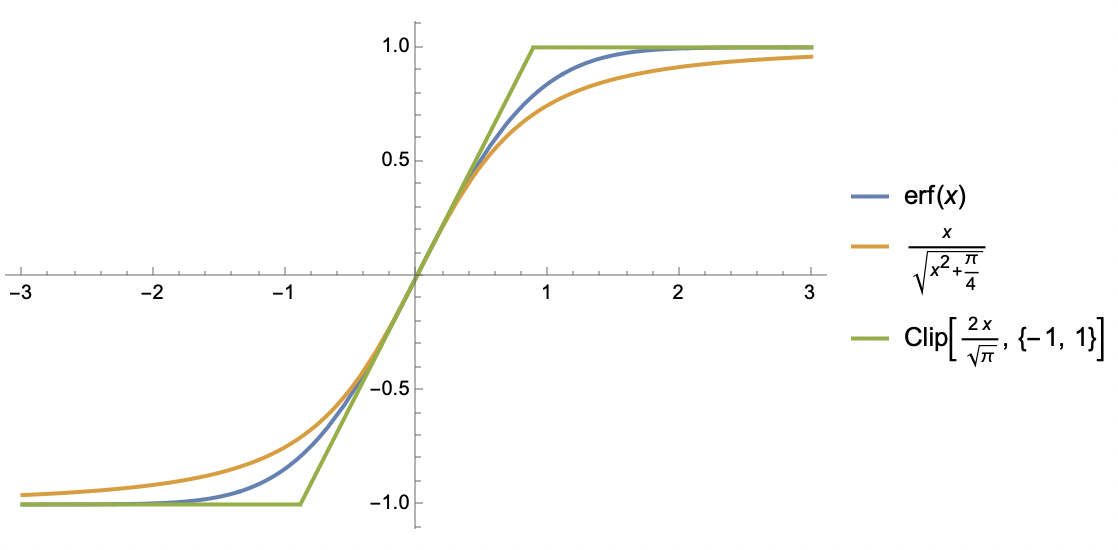
Erf Function and Its Two Approximations

Mean Estimation#

Without delay, following the method from the previous article, the starting point remains:

Our task is to estimate $\mathbb{E}[\tilde{\boldsymbol{\varphi}}_B]$ and $\mathbb{E}[\tilde{\boldsymbol{\varphi}}_B\tilde{\boldsymbol{\varphi}}_B^{\top}]$.

In this section, we compute $\mathbb{E}[\tilde{\boldsymbol{\varphi}}_B]$. For this, we need to approximate the $\text{softsign}$ function using the $\text{clip}$ function:

Then we have:

The integral form is complex, but it's not difficult to compute with Mathematica. The result can be expressed using the $\text{erf}$ function:

where $a = g\sqrt{B}/\sigma, b=\epsilon \sqrt{B}/\sigma$. This function appears rather complicated, but it happens to be an S-shaped function of $a$, with range $(-1,1)$ and slope at $a=0$ equal to $\text{erf}(b/\sqrt{2})/b$. Therefore, using the first approximation form:

The second approximation uses $\text{erf}(x)\approx x / \sqrt{x^2 + \pi / 4}$ to handle $\text{erf}(b/\sqrt{2})$ in the denominator. We can consider ourselves quite fortunate, as the final form is not overly complicated. Then we have:

Similar to the previous article, the last approximation employs a mean field approximation, where $\kappa^2$ is some average of all $\sigma_i^2 /(g_i^2+\epsilon^2)$, and $\nu_i = \text{softsign}(g_i, \epsilon)$ and $\beta = (1 + \pi\kappa^2 / 2B)^{-1/2}$.

Variance Estimation#

Having addressed the mean (first moment), we now turn to the second moment:

The result can also be expressed using $\text{erf}$ functions, but it is even more verbose, so we won't write it out here. As before, for Mathematica, this is no issue. When viewed as a function of $a$, the result is an inverted bell-shaped curve symmetric about the y-axis, with an upper bound of 1 and a minimum within $(0,1)$. Referring to the approximation (9) for $\mathbb{E}[\tilde{\varphi}_B]$, we choose the following approximation:

To be honest, this approximation is not highly accurate, primarily for computational convenience. However, it retains key characteristics: inverted bell shape, y-axis symmetry, upper bound of 1, result of 1 when $b=0$, and result approaching 0 as $b\to\infty$. Next, we continue applying the mean field approximation:

Thus, $\mathbb{E}[\tilde{\boldsymbol{\varphi}}_B\tilde{\boldsymbol{\varphi}}_B^{\top}]_{i,j}\approx \nu_i \nu_j \beta^2 + \delta_{i,j}(1-\beta^2)$. The term $\delta_{i,j}(1-\beta^2)$ represents the covariance matrix $(1-\beta^2)\boldsymbol{I}$ of $\tilde{\boldsymbol{\varphi}}$, which is diagonal—this is expected because one of our assumptions is independence between components of $\tilde{\boldsymbol{\varphi}}$, so the covariance matrix must be diagonal.

Preliminary Results#

From this, we obtain:

In the previous article, we mentioned that one of Adam's most important characteristics is the possible occurrence of the "Surge phenomenon," where $\eta^*$ is no longer globally monotonically increasing with respect to $B$. Next, we will prove that introducing $\epsilon > 0$ reduces the likelihood of the Surge phenomenon occurring, and it completely disappears as $\epsilon \to \infty$. This proof is not difficult; clearly, a necessary condition for the Surge phenomenon to occur is:

If not, the entire $\eta^*$ is monotonically increasing with respect to $\beta$, and since $\beta$ is monotonically increasing with respect to $B$, $\eta^*$ is monotonically increasing with respect to $B$, and no Surge phenomenon exists. Recall that $\nu_i = \text{softsign}(g_i, \epsilon)$ is a monotonically decreasing function of $\epsilon$, so as $\epsilon$ increases, $\sum_{i,j} \nu_i \nu_j H_{i,j}$ becomes smaller, making the above inequality less likely to hold. As $\epsilon\to \infty$, $\nu_i$ approaches zero, and the inequality can no longer hold, so the Surge phenomenon disappears.

Furthermore, we can prove that as $\epsilon\to\infty$, the result becomes consistent with SGD. This only requires noticing:

We have the limits:

Here, $\sigma^2$ is some average of all $\sigma_i^2$. Thus, we obtain the approximation for sufficiently large $\epsilon$:

Summary#

This article continues the methodology of the previous article, attempting to analyze the impact of Adam's $\epsilon$ on the scaling laws between learning rate and batch size. The result is a form intermediate between SGD and SignSGD: the larger $\epsilon$ is, the closer the result is to SGD, and the lower the probability of the "Surge phenomenon" occurring. Overall, the computational results contain no particularly surprising elements, but they can serve as a reference process for analyzing the role of $\epsilon$.