Muon Optimizer Appreciation: The Essential Leap from Vectors to Matrices

With the advent of the LLM era, academic enthusiasm for optimizer research appears to have waned. This is primarily because the currently mainstream AdamW already meets most requirements, and significantly modifying optimizers incurs substantial validation costs. Therefore, most current optimizer variations are merely minor patches that industry applies to AdamW based on their training experience.

However, an optimizer named "Muon" recently gained significant attention on Twitter. It claims to be more efficient than AdamW and not merely a minor tweak based on Adam but rather embodies some thought-provoking principles about the differences between vectors and matrices. Let's explore it together in this article.

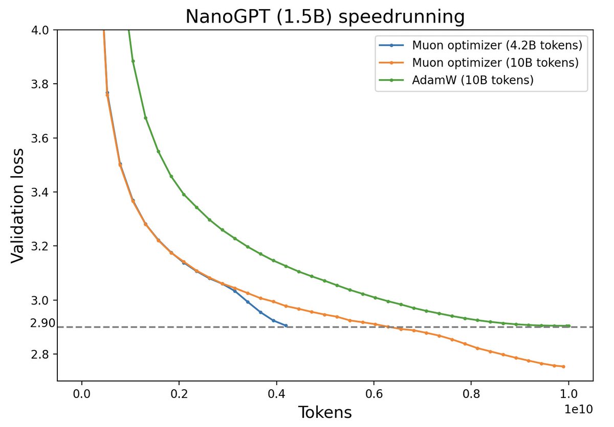
Muon vs AdamW Performance Comparison (Source: Twitter @Yuchenj_UW)

Algorithm Overview#

Muon, short for "MomentUm Orthogonalized by Newton-schulz", is designed for matrix parameters $\boldsymbol{W}\in\mathbb{R}^{n\times m}$. Its update rule is:

Here $\text{msign}$ is the matrix sign function, which is not simply applying $\text{sign}$ element-wise to the matrix but rather a matrix generalization of the $\text{sign}$ function. Its relationship with SVD is:

where $\boldsymbol{U}\in\mathbb{R}^{n\times n},\boldsymbol{\Sigma}\in\mathbb{R}^{n\times m},\boldsymbol{V}\in\mathbb{R}^{m\times m}$, and $r$ is the rank of $\boldsymbol{M}$. We'll elaborate on more theoretical details later, but first, let's intuitively understand the following fact:

Muon is an adaptive learning rate optimizer similar to Adam.

Adaptive learning rate optimizers like Adagrad, RMSprop, and Adam adjust each parameter's update by dividing by the square root of the moving average of gradient squares, achieving two effects: 1. Constant scaling of the loss function doesn't affect the optimization trajectory; 2. Each parameter component's update magnitude is made as consistent as possible. Muon precisely satisfies these two properties:

1. When the loss function is multiplied by $\lambda$, $\boldsymbol{M}$ is also multiplied by $\lambda$, resulting in $\boldsymbol{\Sigma}$ being multiplied by $\lambda$. However, Muon's final update transforms $\boldsymbol{\Sigma}$ into an identity matrix, so it doesn't affect optimization results;

2. When $\boldsymbol{M}$ is decomposed via SVD as $\boldsymbol{U}\boldsymbol{\Sigma}\boldsymbol{V}^{\top}$, different singular values in $\boldsymbol{\Sigma}$ reflect the "anisotropy" of $\boldsymbol{M}$. Setting them all to one makes them more isotropic, also serving to synchronize update magnitudes.

Regarding point 2, did any readers recall BERT-whitening? Additionally, it should be noted that Muon also has a Nesterov version, which simply replaces $\text{msign}(\boldsymbol{M}_t)$ with $\text{msign}(\beta\boldsymbol{M}_t + \boldsymbol{G}_t)$ in the update rule, with all other parts remaining identical. For simplicity, we won't elaborate further.

(Historical note: It was later discovered that the 2015 paper "Stochastic Spectral Descent for Restricted Boltzmann Machines" already proposed an optimization algorithm roughly identical to Muon, then called "Stochastic Spectral Descent.")

Sign Function#

Using SVD, we can also prove the identity:

where ${}^{-1/2}$ is the inverse of the $1/2$ power of the matrix (or the pseudoinverse if not invertible). This identity helps us better understand why $\text{msign}$ is the matrix generalization of $\text{sign}$: for scalar $x$ we have $\text{sign}(x)=x(x^2)^{-1/2}$, which is exactly a special case of the above equation (when $\boldsymbol{M}$ is a $1\times 1$ matrix). This special case can be extended to diagonal matrices $\boldsymbol{M}=\text{diag}(\boldsymbol{m})$:

where $\text{sign}(\boldsymbol{m})$, $\text{sign}(\boldsymbol{M})$ means applying $\text{sign}$ element-wise to the vector/matrix. The above equation implies that when $\boldsymbol{M}$ is diagonal, Muon degenerates to momentum-based SignSGD (Signum) or Tiger proposed by the author, both classical approximations of Adam. Conversely, the difference between Muon and Signum/Tiger is replacing the element-wise $\text{sign}(\boldsymbol{M})$ with the matrix version $\text{msign}(\boldsymbol{M})$.

For an $n$-dimensional vector, we can view it as an $n\times 1$ matrix, where $\text{msign}(\boldsymbol{m}) = \boldsymbol{m}/\Vert\boldsymbol{m}\Vert_2$ is exactly $l_2$ normalization. Therefore, under the Muon framework, we have two perspectives for vectors: first as diagonal matrices (like LayerNorm's gamma parameters), resulting in applying $\text{sign}$ to momentum; second as $n\times 1$ matrices, resulting in $l_2$ normalization of momentum. Additionally, although input and output embeddings are also matrices, they are used sparsely, so a more reasonable approach is to treat them as multiple independent vectors.

When $m=n=r$, $\text{msign}(\boldsymbol{M})$ has another meaning as the "optimal orthogonal approximation":

Similarly, for $\text{sign}(\boldsymbol{M})$ we can write (assuming $\boldsymbol{M}$ has no zero elements):

Whether $\boldsymbol{O}^{\top}\boldsymbol{O} = \boldsymbol{I}$ or $\boldsymbol{O}\in\{-1,1\}^{n\times m}$, we can regard them as regularization constraints on updates. Thus Muon and Signum/Tiger can be viewed as optimizers under the same conceptual framework—they all start from momentum $\boldsymbol{M}$ to construct updates but choose different regularization methods.

Proof of Equation (5): For orthogonal matrix $\boldsymbol{O}$, we have:
\begin{equation}\begin{aligned} \Vert \boldsymbol{M} - \boldsymbol{O}\Vert_F^2 =&\, \Vert \boldsymbol{M}\Vert_F^2 + \Vert \boldsymbol{O}\Vert_F^2 - 2\langle\boldsymbol{M},\boldsymbol{O}\rangle_F \\[5pt] =&\, \Vert \boldsymbol{M}\Vert_F^2 + n - 2\text{Tr}(\boldsymbol{M}\boldsymbol{O}^{\top})\\[5pt] =&\, \Vert \boldsymbol{M}\Vert_F^2 + n - 2\text{Tr}(\boldsymbol{U}\boldsymbol{\Sigma}\boldsymbol{V}^{\top}\boldsymbol{O}^{\top})\\[5pt] =&\, \Vert \boldsymbol{M}\Vert_F^2 + n - 2\text{Tr}(\boldsymbol{\Sigma}\boldsymbol{V}^{\top}\boldsymbol{O}^{\top}\boldsymbol{U})\\ =&\, \Vert \boldsymbol{M}\Vert_F^2 + n - 2\sum_{i=1}^n \boldsymbol{\Sigma}_{i,i}(\boldsymbol{V}^{\top}\boldsymbol{O}^{\top}\boldsymbol{U})_{i,i} \end{aligned}\end{equation}
The involved operational rules have been introduced in pseudoinverse. Since $\boldsymbol{U},\boldsymbol{V},\boldsymbol{O}$ are orthogonal matrices, $\boldsymbol{V}^{\top}\boldsymbol{O}^{\top}\boldsymbol{U}$ is also orthogonal. Orthogonal matrix elements cannot exceed 1, and since $\boldsymbol{\Sigma}_{i,i} > 0$, minimizing the above expression corresponds to maximizing each $(\boldsymbol{V}^{\top}\boldsymbol{O}^{\top}\boldsymbol{U})_{i,i}$, i.e., $(\boldsymbol{V}^{\top}\boldsymbol{O}^{\top}\boldsymbol{U})_{i,i}=1$, which means $\boldsymbol{V}^{\top}\boldsymbol{O}^{\top}\boldsymbol{U}=\boldsymbol{I}$, i.e., $\boldsymbol{O}=\boldsymbol{U}\boldsymbol{V}^{\top}$.

This conclusion can be carefully extended to cases where $m,n,r$ are unequal but won't be further expanded here.

Iterative Solution#

In practice, if we perform SVD on $\boldsymbol{M}$ at each step to compute $\text{msign}(\boldsymbol{M})$, the computational cost would be substantial. Therefore, the author proposes using Newton-Schulz iteration to approximate $\text{msign}(\boldsymbol{M})$.

The iteration starts from identity (3). Without loss of generality, assume $n\geq m$, then consider Taylor expanding $(\boldsymbol{M}^{\top}\boldsymbol{M})^{-1/2}$ around $\boldsymbol{M}^{\top}\boldsymbol{M}=\boldsymbol{I}$. The expansion method is directly applying the scalar function $t^{-1/2}$ result to the matrix:

Keeping up to second order gives $(15 - 10t + 3t^2)/8$, so we have:

If $\boldsymbol{X}_t$ is some approximation of $\text{msign}(\boldsymbol{M})$, substituting it into the above should yield a better approximation of $\text{msign}(\boldsymbol{M})$, giving us a usable iterative scheme:

However, examining Muon's official code reveals that its Newton-Schulz iteration indeed has this form, but the three coefficients are $(3.4445, -4.7750, 2.0315)$, with no mathematical derivation provided by the author, only cryptic comments:

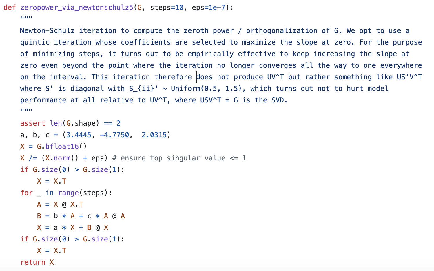
Muon Optimizer's Newton-Schulz Iteration

Convergence Acceleration#

To guess the origin of the official iterative algorithm, consider a general iteration process:

where $a,b,c$ are three coefficients to be determined. For higher-order iterative algorithms, we can sequentially add terms like $\boldsymbol{X}_t(\boldsymbol{X}_t^{\top}\boldsymbol{X}_t)^3$, $\boldsymbol{X}_t(\boldsymbol{X}_t^{\top}\boldsymbol{X}_t)^4$, etc. The following analysis process is general.

We choose initial value $\boldsymbol{X}_0=\boldsymbol{M}/\Vert\boldsymbol{M}\Vert_F$, where $\Vert\cdot\Vert_F$ is the matrix $F$-norm. The rationale is dividing by $\Vert\boldsymbol{M}\Vert_F$ doesn't change SVD's $\boldsymbol{U},\boldsymbol{V}$ but ensures all singular values of $\boldsymbol{X}_0$ are in $[0,1]$, making initial singular values more standardized. Assuming $\boldsymbol{X}_t$ can be SVD decomposed as $\boldsymbol{U}\boldsymbol{\Sigma}_t\boldsymbol{V}^{\top}$, substituting into the above gives:

Thus, Equation (10) actually iterates the diagonal matrix $\boldsymbol{\Sigma}_{[:r,:r]}$ composed of singular values. If we denote $\boldsymbol{X}_t=\boldsymbol{U}_{[:,:r]}\boldsymbol{\Sigma}_{t,[:r,:r]}\boldsymbol{V}_{[:,:r]}^{\top}$, then $\boldsymbol{\Sigma}_{t+1,[:r,:r]} = g(\boldsymbol{\Sigma}_{t,[:r,:r]})$, where $g(x) = ax + bx^3 + cx^5$. Since powers of diagonal matrices equal element-wise powers, the problem simplifies to iterating individual singular values $\sigma$. Our goal is to compute $\boldsymbol{U}_{[:,:r]}\boldsymbol{V}_{[:,:r]}^{\top}$, i.e., to transform $\boldsymbol{\Sigma}_{[:r,:r]}$ into an identity matrix via iteration, which simplifies to iterating $\sigma_{t+1} = g(\sigma_t)$ to transform a single singular value to 1.

Inspired by @leloykun, we treat selecting $a,b,c$ as an optimization problem aiming for the fastest possible convergence for arbitrary initial singular values. First, reparameterize $g(x)$ as:

where $x_1 \leq x_2$. This parameterization intuitively shows the iteration's five fixed points $0,\pm x_1,\pm x_2$. Since our goal is convergence to 1, we choose initialization with $x_1 < 1, x_2 > 1$, hoping iteration moves toward $x_1$ or $x_2$, both near 1.

Next, determine iteration steps $T$, making the iteration process a deterministic function. Then fix matrix shape ($n,m$) and sample a batch of matrices, compute singular values via SVD. Finally, treat these singular values as input, target output as 1, loss function as squared error. The entire model is fully differentiable and solvable via gradient descent (@leloykun assumed $x_1 + x_2 = 2$ and used grid search).

Some calculation results:

n    m    T    κ      x₁    x₂    a      b       c      mse    mseₒ
1024 1024 3    7.020  0.830 0.830 4.328  -9.666  7.020  0.10257 0.18278
1024 1024 5    1.724  0.935 1.235 3.297  -4.136  1.724  0.02733 0.04431
2048 1024 3    7.028  0.815 0.815 4.095  -9.327  7.028  0.01628 0.06171
2048 1024 5    1.476  0.983 1.074 2.644  -3.128  1.476  0.00038 0.02954
4096 1024 3    6.948  0.802 0.804 3.886  -8.956  6.948  0.00371 0.02574
4096 1024 5    1.214  1.047 1.048 2.461  -2.663  1.214  0.00008 0.02563
2048 2048 3    11.130 0.767 0.767 4.857  -13.103 11.130 0.10739 0.24410
2048 2048 5    1.779  0.921 1.243 3.333  -4.259  1.779  0.03516 0.04991
4096 4096 3    18.017 0.705 0.705 5.460  -17.929 18.017 0.11303 0.33404
4096 4096 5    2.057  0.894 1.201 3.373  -4.613  2.057  0.04700 0.06372
8192 8192 3    30.147 0.643 0.643 6.139  -24.893 30.147 0.11944 0.44843
8192 8192 5    2.310  0.871 1.168 3.389  -4.902  2.310  0.05869 0.07606

Here $\text{mse}_{\text{o}}$ is the result calculated using Muon author's $a,b,c$. The table shows results clearly depend on matrix size and iteration steps; from loss perspective, non-square matrices converge more easily than square ones; Muon author's $a,b,c$ roughly correspond to square matrices' optimal solution for $T=5$. Given iteration steps, results depend on matrix size, essentially depending on singular value distribution. A noteworthy result about this distribution is the Marchenko–Pastur distribution when $n,m\to\infty$.

Reference code:

import jax
import jax.numpy as jnp
from tqdm import tqdm

n, m, T = 1024, 1024, 5
key, data = jax.random.key(42), jnp.array([])
for _ in tqdm(range(1000), ncols=0, desc='SVD'):
    key, subkey = jax.random.split(key)
    M = jax.random.normal(subkey, shape=(n, m))
    S = jnp.linalg.svd(M, full_matrices=False)[1]
    data = jnp.concatenate([data, S / (S**2).sum()**0.5])

@jax.jit
def f(w, x):
    k, x1, x2 = w
    for _ in range(T):
        x = x + k * x * (x**2 - x1**2) * (x**2 - x2**2)
    return ((x - 1)**2).mean()

f_grad = jax.grad(f)
w, u = jnp.array([1, 0.9, 1.1]), jnp.zeros(3)
for _ in tqdm(range(100000), ncols=0, desc='SGD'):
    u = 0.9 * u + f_grad(w, data)  # momentum acceleration
    w = w - 0.01 * u

k, x1, x2 = w
a, b, c = 1 + k * x1**2 * x2**2, -k * (x1**2 + x2**2), k
print(f'{n} & {m} & {T} & {k:.3f} & {x1:.3f} & {x2:.3f} & {a:.3f} & {b:.3f} & {c:.3f} & {f(w, data):.5f}')

Deeper Thoughts#

With default $T=5$, for an $n\times n$ matrix parameter, each Muon update requires at least 15 multiplications of $n\times n$ with $n\times n$ matrices. This computational load is undoubtedly significantly larger than Adam, raising concerns about Muon's practical feasibility.

In fact, this concern is unwarranted. Although Muon's computation is more complex than Adam, the time increase per step is minimal—the author's conclusion is within 5%, while Muon's author claims 2%. This is because Muon's matrix multiplications occur after current gradient computation and before next gradient computation, when almost all computing power is idle. These matrix multiplications have static sizes and can be parallelized, so they don't significantly increase time costs. Instead, Muon has one less cached variable than Adam, resulting in lower memory costs.

The most thought-provoking aspect of Muon is the intrinsic difference between vectors and matrices and its impact on optimization. Common optimizers like SGD, Adam, and Tiger have element-wise update rules, treating all parameters (vectors or matrices) as one large vector with components updated independently according to identical rules. Optimizers with this characteristic tend to simplify theoretical analysis and facilitate tensor parallelism, as splitting a large matrix into smaller independent matrices doesn't change optimization trajectories.

But Muon is different—it treats matrices as fundamental units, considering unique matrix characteristics. Some readers might wonder: aren't matrices and vectors just arrangements of numbers? What's the difference? For example, matrices have the concept of "trace"—the sum of diagonal elements. This isn't arbitrarily defined; it has an important property of being invariant under similarity transformations and equals the sum of all matrix eigenvalues. This example shows diagonal and off-diagonal elements don't have completely equal status. Muon's superior performance stems precisely from considering this inequality.

Of course, this also introduces negative consequences. If a matrix is partitioned across different devices, Muon requires gathering their gradients to compute updates rather than each device updating independently, increasing communication costs. Even without considering parallelism, this issue exists. For example, Multi-Head Attention typically projects through a single large matrix to $Q$ (similarly for $K,V$), then uses reshape to obtain multiple heads. Thus, model parameters contain only a single matrix, but it essentially comprises multiple small matrices, so theoretically we should split the large matrix into multiple small matrices for independent updates.

In summary, Muon's non-element-wise update rules capture essential differences between vectors and matrices while introducing minor issues that might dissatisfy some readers aesthetically.

(Addition: Almost simultaneously with this blog post's publication, Muon author Keller Jordan published his own blog "Muon: An optimizer for hidden layers in neural networks".)

Norm Perspective#

Theoretically, what key matrix characteristics does Muon capture? Perhaps the following norm perspective can answer our question.

This section's discussion mainly references papers "Stochastic Spectral Descent for Discrete Graphical Models" and "Old Optimizer, New Norm: An Anthology", particularly the latter. However, the starting point isn't new; we briefly touched on it in "Gradient Flow: Exploring Paths to Minima": For vector parameters $\boldsymbol{w}\in\mathbb{R}^n$, define next-step update rule as:

where $\Vert\Vert$ is some vector norm. This is called "steepest gradient descent" under some norm constraint. Assuming $\eta_t$ is sufficiently small, the first term dominates, meaning $\boldsymbol{w}_{t+1}$ is close to $\boldsymbol{w}_t$, so we assume $\mathcal{L}(\boldsymbol{w})$'s first-order approximation suffices, simplifying the problem to:

Let $\Delta\boldsymbol{w}_{t+1} = \boldsymbol{w}_{t+1}-\boldsymbol{w}_t, \boldsymbol{g}_t = \nabla_{\boldsymbol{w}_t}\mathcal{L}(\boldsymbol{w}_t)$, then simplified as:

The general approach for computing $\Delta\boldsymbol{w}_{t+1}$ is differentiation, but "Old Optimizer, New Norm: An Anthology" provides a unified scheme without differentiation: Decompose $\Delta\boldsymbol{w}$ into norm $\gamma = \Vert\Delta\boldsymbol{w}\Vert$ and direction vector $\boldsymbol{\varphi} = -\Delta\boldsymbol{w}/\Vert\Delta\boldsymbol{w}\Vert$, then:

$\gamma$ is just a scalar, similar to learning rate, easily found optimal as $\eta_t\Vert \boldsymbol{g}_t\Vert^{\dagger}$, while update direction is $\boldsymbol{\varphi}^*$ maximizing $\boldsymbol{g}_t^{\top}\boldsymbol{\varphi}$ ($\Vert\boldsymbol{\varphi}\Vert=1$). Substituting Euclidean norm $\Vert\boldsymbol{\varphi}\Vert_2 = \sqrt{\boldsymbol{\varphi}^{\top}\boldsymbol{\varphi}}$ gives $\Vert \boldsymbol{g}_t\Vert^{\dagger}=\Vert \boldsymbol{g}_t\Vert_2$ and $\boldsymbol{\varphi}^* = \boldsymbol{g}_t/\Vert\boldsymbol{g}_t\Vert_2$, yielding $\Delta\boldsymbol{w}_{t+1}=-\eta_t \boldsymbol{g}_t$, i.e., gradient descent (SGD). Generally, for $p$-norm:

Hölder's inequality gives $\boldsymbol{g}^{\top}\boldsymbol{\varphi} \leq \Vert \boldsymbol{g}\Vert_q \Vert \boldsymbol{\varphi}\Vert_p$, where $1/p + 1/q = 1$, giving us:

Equality holds when:

Optimizers using this direction vector are called pbSGD, refer to "pbSGD: Powered Stochastic Gradient Descent Methods for Accelerated Non-Convex Optimization". Particularly, when $p\to\infty$, $q\to 1$ and $|g_i|^{q/p}\to 1$, degenerating to SignSGD, i.e., SignSGD is actually steepest gradient descent under $\Vert\Vert_{\infty}$ norm.

Matrix Norms#

Now shift focus to matrix parameters $\boldsymbol{W}\in\mathbb{R}^{n\times m}$. Similarly, define its update rule as:

Here $\Vert\Vert$ is some matrix norm. Using first-order approximation gives:

where $\Delta\boldsymbol{W}_{t+1} = \boldsymbol{W}_{t+1}-\boldsymbol{W}_t, \boldsymbol{G}_t = \nabla_{\boldsymbol{W}_t}\mathcal{L}(\boldsymbol{W}_t)$. Still using "norm-direction" decoupling, i.e., set $\gamma = \Vert\Delta\boldsymbol{w}\Vert$ and $\boldsymbol{\Phi} = -\Delta\boldsymbol{W}/\Vert\Delta\boldsymbol{W}\Vert$, we get:

Then analyze specific norms. Two common matrix norms: one is the F-norm, which essentially computes Euclidean norm after flattening matrix to vector—conclusions match vectors, answer is SGD, not elaborated here; the other is the $2$-norm induced from vector norms, also called spectral norm:

Note $\Vert\Vert_2$ in the right side applies to vectors, so definition is clear. More discussion about $2$-norm can be found in "Lipschitz Constraints in Deep Learning: Generalization and Generative Models" and "The Path to Low-Rank Approximation (II): SVD". Since $2$-norm is induced by "matrix-vector" multiplication, it better aligns with matrix multiplication, and always satisfies $\Vert\boldsymbol{\Phi}\Vert_2\leq \Vert\boldsymbol{\Phi}\Vert_F$, i.e., $2$-norm is more compact than F-norm.

So, next compute for $2$-norm specifically. Let $\boldsymbol{G}$'s SVD be $\boldsymbol{U}\boldsymbol{\Sigma}\boldsymbol{V}^{\top} = \sum\limits_{i=1}^r \sigma_i \boldsymbol{u}_i \boldsymbol{v}_i^{\top}$, we have:

By definition, when $\Vert\boldsymbol{\Phi}\Vert_2=1$, $\Vert\boldsymbol{\Phi}\boldsymbol{v}_i\Vert_2\leq \Vert\boldsymbol{v}_i\Vert_2=1$, so $\boldsymbol{u}_i^{\top}\boldsymbol{\Phi}\boldsymbol{v}_i\leq 1$, therefore:

Equality holds when all $\boldsymbol{u}_i^{\top}\boldsymbol{\Phi}\boldsymbol{v}_i$ equal 1, then:

Thus we've proven gradient descent under $2$-norm penalty is exactly the Muon optimizer with $\beta=0$! When $\beta > 0$, moving average takes effect, which can be viewed as a more accurate gradient estimate, so changed to applying $\text{msign}$ to momentum. Overall, Muon corresponds to gradient descent under $2$-norm constraint, where $2$-norm better measures essential differences between matrices, making each step more precise and fundamental.

Historical Context#

Muon has an older related work "Shampoo: Preconditioned Stochastic Tensor Optimization", a 2018 paper proposing the Shampoo optimizer, sharing similarities with Muon.

Adam's strategy of adapting learning rates via moving averages of gradient squares originated from Adagrad's paper "Adaptive Subgradient Methods for Online Learning and Stochastic Optimization", which proposed directly accumulating gradient squares—equivalent to global equal-weight averaging. Later RMSProp and Adam, inspired by momentum design, changed to moving averages, performing better in practice.

Moreover, Adagrad originally proposed accumulating outer products $\boldsymbol{g}\boldsymbol{g}^{\top}$, but caching outer products was too costly in space, so practice switched to Hadamard products $\boldsymbol{g}\odot\boldsymbol{g}$. What's the theoretical basis for accumulating outer products? As derived in "Viewing Adaptive Learning Rate Optimizers from Hessian Approximation", the answer is "long-term average of gradient outer products $\mathbb{E}[\boldsymbol{g}\boldsymbol{g}^{\top}]$ approximates Hessian matrix square $\sigma^2\boldsymbol{\mathcal{H}}_{\boldsymbol{\theta}^*}^2$", so this actually approximates second-order Newton's method.

Shampoo inherits Adagrad's idea of caching outer products but compromises considering cost. Like Muon, it optimizes matrices (and higher-order tensors), strategy being caching gradient matrix products $\boldsymbol{G}\boldsymbol{G}^{\top}$ and $\boldsymbol{G}^{\top}\boldsymbol{G}$, not outer products, with space cost $\mathcal{O}(n^2 + m^2)$ instead of $\mathcal{O}(n^2 m^2)$:

Here $\beta$ is added by the author; Shampoo defaults $\beta=1$. ${}^{-1/4}$ is again matrix power operations, computable via SVD. Since Shampoo didn't propose approximate schemes like Newton-Schulz iteration but directly uses SVD, to save computation costs, it doesn't compute $\boldsymbol{L}_t^{-1/4}$ and $\boldsymbol{R}_t^{-1/4}$ every step but updates them periodically.

Particularly, when $\beta=0$, Shampoo's update vector is $(\boldsymbol{G}\boldsymbol{G}^{\top})^{-1/4}\boldsymbol{G}(\boldsymbol{G}^{\top}\boldsymbol{G})^{-1/4}$. Through SVD of $\boldsymbol{G}$ we can prove:

This shows Shampoo and Muon are theoretically equivalent when $\beta=0$! Therefore, Shampoo and Muon share common ground in update design.

Summary#

This article introduces the recently popular Muon optimizer on Twitter. It's specifically designed for matrix parameters, currently appears more efficient than AdamW, and seems to embody some essential differences between vectorization and matrixization, worthy of study and reflection.