Muon Sequel: Why We Chose to Experiment with Muon?

This article interprets our latest technical report "Muon is Scalable for LLM Training", which shares our large-scale practice with the Muon optimizer previously introduced in "Muon Optimizer Appreciation: The Essential Leap from Vectors to Matrices", and open-sources the corresponding model (we call it "Moonlight", currently a 3B/16B MoE model). We discovered a rather surprising conclusion: under our experimental setup, Muon achieves nearly 2x training efficiency compared to Adam.

Muon's Scaling Law and Moonlight's MMLU Performance

There aren't too many optimizer developments, but there are certainly some. Why did we choose Muon as a new experimental direction? How can we quickly transition from a well-tuned Adam optimizer to Muon for experimentation? How do Muon and Adam compare in performance when scaling up models? We will share our thought process next.

Optimization Principles#

Regarding optimizers, the author previously commented in "Muon Optimizer Appreciation: The Essential Leap from Vectors to Matrices" that most optimizer improvements are essentially minor patches—not entirely worthless but ultimately failing to convey a sense of depth or amazement.

We need to consider what constitutes a good optimizer from more fundamental principles. Intuitively, an ideal optimizer should possess two characteristics: stability and speed. Specifically, each step of an ideal optimizer should satisfy two points: 1. Minimize model perturbation; 2. Maximize loss reduction. More directly, we don't want major model changes (stability), yet we want substantial loss reduction (speed)—a classic "both...and..." scenario.

How do we translate these characteristics into mathematical language? Stability can be understood as a constraint on the update magnitude, while speed can be interpreted as finding the update that most rapidly decreases the loss function. This transforms into a constrained optimization problem. Using previous notation, for matrix parameter $\boldsymbol{W}\in\mathbb{R}^{n\times m}$ with gradient $\boldsymbol{G}\in\mathbb{R}^{n\times m}$, when the parameter changes from $\boldsymbol{W}$ to $\boldsymbol{W}+\Delta\boldsymbol{W}$, the loss function change is:

Thus, seeking the fastest update under stable conditions can be expressed as:

Here, $\rho(\Delta\boldsymbol{W})\geq 0$ is some metric of stability, where smaller values indicate greater stability, and $\eta$ is a constant less than 1 representing our requirement for stability. Later we will see this is essentially the optimizer's learning rate. If readers don't mind, we can mimic theoretical physics concepts and call this principle the optimizer's "Least Action Principle".

Matrix Norms#

The only uncertainty in Equation (2) is the stability metric $\rho(\Delta\boldsymbol{W})$. Once $\rho(\Delta\boldsymbol{W})$ is selected, $\Delta\boldsymbol{W}$ can be explicitly solved (at least theoretically). To some extent, we can consider the fundamental difference between optimizers as their varying definitions of stability.

Many readers likely encountered statements like "the negative gradient direction is the direction of steepest local descent" when first learning SGD. In this framework, it simply chooses the matrix $F$-norm $\Vert\Delta\boldsymbol{W}\Vert_F$ as the stability metric. That is, "the direction of steepest descent" isn't immutable; it's determined only after selecting the metric. With a different norm, it might not be the negative gradient direction.

The natural question is: which norm most appropriately measures stability? If we impose strong constraints, stability is achieved, but the optimizer struggles, converging only to suboptimal solutions. Conversely, weak constraints allow the optimizer to run wild, making training extremely unpredictable. Thus, the ideal scenario is finding the most precise metric for stability. Considering neural networks primarily involve matrix multiplication, take $\boldsymbol{y}=\boldsymbol{x}\boldsymbol{W}$ as an example:

This equation means when parameters change from $\boldsymbol{W}$ to $\boldsymbol{W}+\Delta\boldsymbol{W}$, the model output change is $\Delta\boldsymbol{y}$. We hope this change's magnitude can be controlled by $\Vert\boldsymbol{x}\Vert$ and a function $\rho(\Delta\boldsymbol{W})$ related to $\Delta\boldsymbol{W}$, which we use as the stability metric. From linear algebra, $\rho(\Delta\boldsymbol{W})$'s most accurate value is $\Delta\boldsymbol{W}$'s spectral norm $\Vert\Delta\boldsymbol{W}\Vert_2$. Substituting into Equation (2):

Solving this optimization problem yields Muon with $\beta=0$:

When $\beta > 0$, $\boldsymbol{G}$ is replaced by momentum $\boldsymbol{M}$, which can be viewed as a smoother estimate of the gradient. Thus, the conclusion still holds. Therefore, we can assert that "Muon is the steepest descent under the spectral norm." Details like Newton-Schulz iteration are computational approximations and won't be elaborated here. The detailed derivation was provided in "Muon Optimizer Appreciation: The Essential Leap from Vectors to Matrices" and won't be repeated.

Weight Decay#

Thus far, we can answer the first question: Why choose Muon for experimentation? Like SGD, Muon also provides the direction of steepest descent, but its spectral norm constraint is more precise than SGD's $F$-norm, giving it greater potential. Additionally, improving optimizers from the perspective of "selecting the most appropriate constraints for different parameters" seems more fundamental than various patch-like modifications.

However, potential doesn't guarantee capability. Validating Muon on larger models presents several "traps." First is the Weight Decay problem. Although we included Weight Decay when introducing Muon in "Muon Optimizer Appreciation: The Essential Leap from Vectors to Matrices", the original Muon proposal lacked it. Initially implementing the official version, we found Muon converged quickly early on but was soon caught by Adam, with various "internal issues" showing signs of collapse.

We quickly realized this might be a Weight Decay issue and added it:

Continuing experiments, as expected, Muon now maintained its lead over Adam, as shown in the paper's Figure 2:

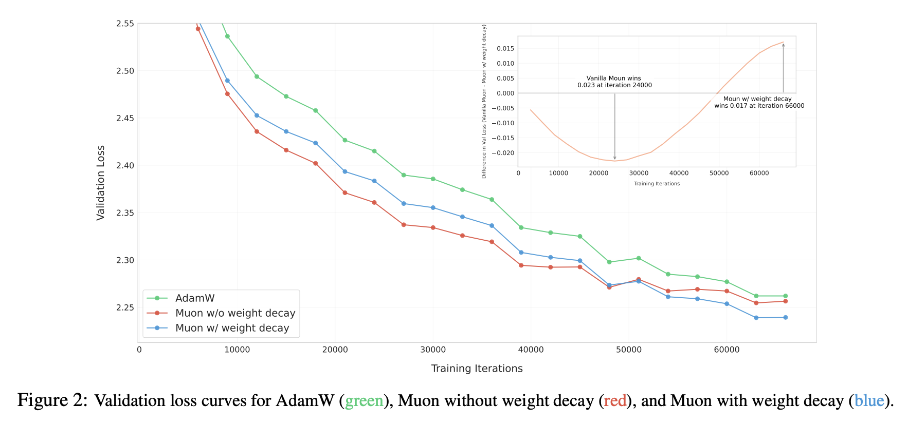
Performance Comparison With and Without Weight Decay

What role does Weight Decay play? Post-analysis suggests a key function may be keeping parameter norms bounded:

Here $\Vert\cdot\Vert$ is any matrix norm—the inequality holds for any matrix norm. $\boldsymbol{\Phi}_t$ is the update vector provided by the optimizer; for Muon, it's $\text{msign}(\boldsymbol{M})$. Taking the spectral norm, $\Vert\text{msign}(\boldsymbol{M})\Vert_2 = 1$. Thus for Muon:

This ensures model "internal health" because $\Vert\boldsymbol{x}\boldsymbol{W}\Vert\leq \Vert\boldsymbol{x}\Vert\Vert\boldsymbol{W}\Vert_2$. Controlling $\Vert\boldsymbol{W}\Vert_2$ means controlling $\Vert\boldsymbol{x}\boldsymbol{W}\Vert$, preventing explosion risks—particularly important for issues like Attention Logits explosion. This bound remains relatively loose in most cases; in practice, parameter spectral norms are often significantly smaller than this bound. This inequality simply shows Weight Decay's norm-controlling property.

RMS Alignment#

When deciding to experiment with a new optimizer, a major headache is quickly finding near-optimal hyperparameters. For Muon, there are at least two: learning rate $\eta_t$ and decay rate $\lambda$. Grid search is possible but time-consuming. Here we propose an Update RMS alignment hyperparameter transfer strategy, enabling reuse of Adam-tuned hyperparameters in other optimizers.

First, for a matrix $\boldsymbol{W}\in\mathbb{R}^{n\times m}$, its RMS (Root Mean Square) is defined as:

Simply put, RMS measures the average magnitude of each matrix element. We observe that Adam's update RMS is relatively stable, typically between 0.2 and 0.4, which is why theoretical analysis often uses SignSGD as an Adam approximation. Based on this, we suggest aligning new optimizers' Update RMS to 0.2 via RMS Norm:

This allows reuse of Adam's $\eta_t$ and $\lambda$, achieving roughly equivalent parameter update magnitudes per step. Practice shows this simple strategy from Adam to Muon yields results significantly better than Adam, approaching those from further Muon hyperparameter fine-tuning. Notably, Muon's $\text{RMS}(\boldsymbol{\Phi}_t)=\text{RMS}(\boldsymbol{U}_{[:,:r]}\boldsymbol{V}_{[:,:r]}^{\top})$ can be computed analytically:

Thus $\text{RMS}(\boldsymbol{\Phi}_t) = \sqrt{r/nm}$. In practice, the probability of a matrix being strictly low-rank is small, so we consider $r = \min(n,m)$, yielding $\text{RMS}(\boldsymbol{\Phi}_t) = \sqrt{1/\max(n,m)}$. Therefore, we ultimately used the equivalent analytic version instead of RMS Norm:

This final equation indicates that in Muon, using a single learning rate for all parameters is inappropriate. For example, Moonlight is an MoE model with many matrix parameter shapes deviating from square matrices, with $\max(n,m)$ spanning a wide range. A single learning rate would inevitably cause asynchronous learning—some parameters learning too fast or too slow—affecting final performance.

Experimental Analysis#

We conducted thorough comparisons between Adam and Muon on 2.4B/16B MoE models, finding Muon significantly outperforms in both convergence speed and final results. For detailed comparisons, we recommend reading the original paper; here we share only partial insights.

Github: https://github.com/MoonshotAI/Moonlight

First is a relatively objective comparison table, including our controlled variable training comparisons between Muon and Adam, and comparisons with externally (DeepSeek) Adam-trained models of identical architecture (for fairness, Moonlight's architecture matches DSV3-Small exactly), highlighting Muon's unique advantages:

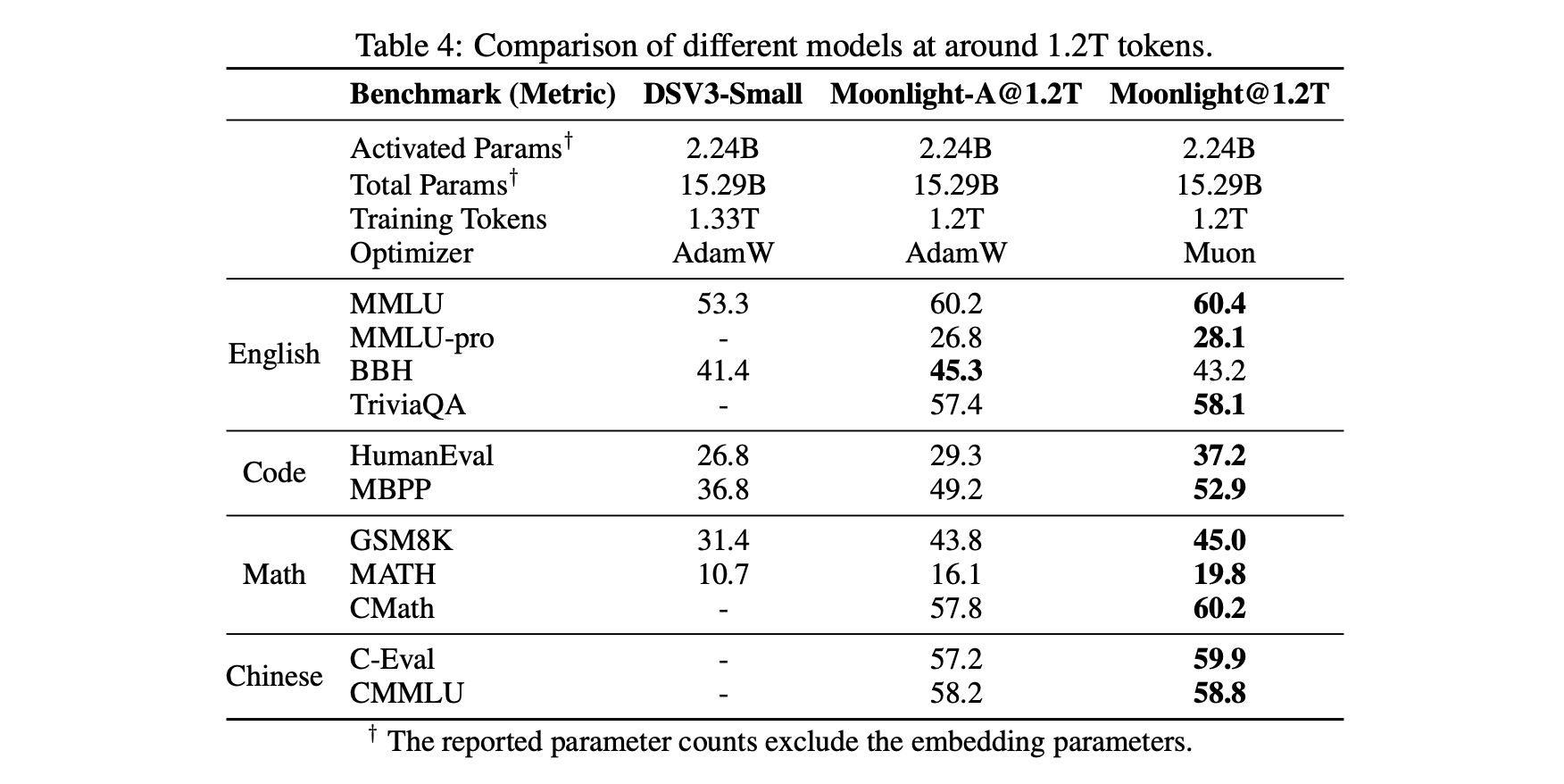
Muon (Moonlight) vs Adam (Moonlight-A and DSV3-small) Comparison

How do Muon-trained models differ? Since we earlier stated Muon is steepest descent under the spectral norm—where the spectral norm is the largest singular value—we considered monitoring and analyzing singular values. Indeed, we found interesting signals: parameters trained with Muon exhibit relatively more uniform singular value distributions. We use singular value entropy to quantify this phenomenon:

Here $\boldsymbol{\sigma}=(\sigma_1,\sigma_2,\cdots,\sigma_n)$ are all singular values of a parameter. Muon-trained parameters have higher entropy—more uniform singular value distributions—meaning parameters are less compressible. This indicates Muon more fully utilizes parameter potential:

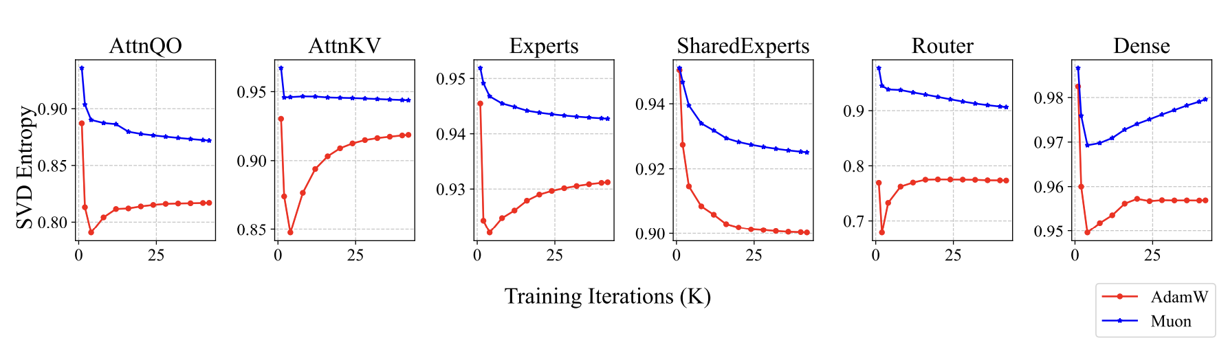
Muon-Trained Weights Have Higher Singular Value Entropy

Another interesting discovery: using Muon for fine-tuning (SFT) might yield suboptimal solutions if pre-training didn't use Muon. Specifically, if both pre-training and fine-tuning use Muon, performance is best. But for the other three combinations (Adam+Muon, Muon+Adam, Adam+Adam), performance superiority doesn't show clear patterns.

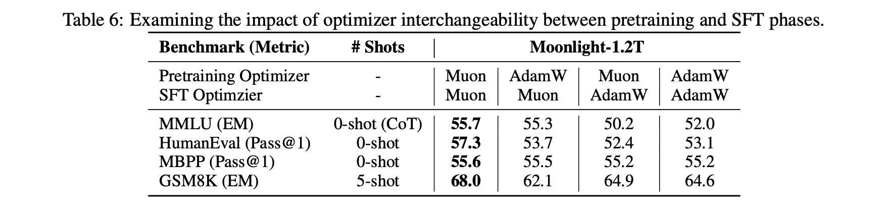
Pre-training/Fine-tuning Combinations Test (Muon/Adam)

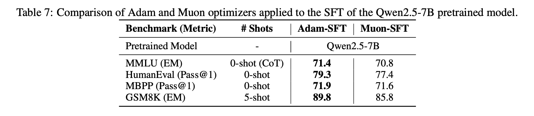
Attempts to Fine-Tune Open-Source Models with Muon/Adam

This phenomenon suggests certain initializations are unfavorable for Muon—conversely, some may be more favorable. We are still exploring underlying principles.

Extended Thoughts#

Overall, in our experiments, Muon's performance appears highly competitive compared to Adam. As a new optimizer with significantly different formulation from Adam, this performance isn't merely "commendable"; it suggests Muon may capture some essential characteristics.

Previously, the community circulated a view: Adam performs well because mainstream model architecture improvements have been "overfitting" to Adam. This view likely originated from "Neural Networks (Maybe) Evolved to Make Adam The Best Optimizer", seemingly absurd but profoundly meaningful. Consider: when we attempt model improvements, we train with Adam to evaluate performance; good results are retained, otherwise abandoned. But does good performance stem from inherent superiority or better compatibility with Adam?

This is thought-provoking. Certainly, at least some work shows better performance because it matches Adam better, so over time, model architectures evolve toward directions favorable to Adam. In this context, an optimizer significantly different from Adam still "breaking through" deserves particular attention and reflection. Note that the author and affiliated company are not Muon's proposers, so these remarks are sincere without self-promotion.

What work remains for Muon? Actually, quite a bit. For example, the "Adam pre-training + Muon fine-tuning" performance issue mentioned above warrants further analysis—valuable and necessary, especially since most open-source model weights are Adam-trained. If Muon fine-tuning fails, it inevitably hinders adoption. We can also deepen understanding of Muon through this opportunity (learning through bugs).

Another extension consideration: Muon is based on the spectral norm—the largest singular value. In fact, we can construct a series of norms based on singular values, like Schatten norms. Extending to these broader norms and tuning parameters could theoretically yield better results. Additionally, after Moonlight's release, some readers asked how to design µP (maximal update parametrization) under Muon—another urgent problem to solve.

Summary#

This article introduces our large-scale practice with the Muon optimizer (Moonlight) and shares our latest reflections on the Muon optimizer.