In the previous article, we introduced the "Pseudo-Inverse", which relates to the optimal solution of the optimization objective \(\Vert \boldsymbol{A}\boldsymbol{B} - \boldsymbol{M}\Vert_F^2\) when given matrices \(\boldsymbol{M}\) and \(\boldsymbol{A}\) (or \(\boldsymbol{B}\)). In this article, we focus on the optimal solution when neither \(\boldsymbol{A}\) nor \(\boldsymbol{B}\) is given:
where \(\boldsymbol{A}\in\mathbb{R}^{n\times r}, \boldsymbol{B}\in\mathbb{R}^{r\times m}, \boldsymbol{M}\in\mathbb{R}^{n\times m}, r < \min(n,m)\). Essentially, this seeks the "optimal rank-\(r\) approximation of matrix \(\boldsymbol{M}\)" (the best approximation with rank at most \(r\)). To solve this problem, we must invoke the celebrated "SVD (Singular Value Decomposition)." Although this series began with the pseudo-inverse, its "fame" pales in comparison to SVD. Many have heard of or even used SVD without encountering the pseudo-inverse, including the author, who learned SVD first before encountering the pseudo-inverse.
Next, we will introduce SVD centered around the theme of optimal low-rank approximation of matrices.
Initial Exploration#
For any matrix \(\boldsymbol{M}\in\mathbb{R}^{n\times m}\), we can find a Singular Value Decomposition (SVD) of the following form:
where \(\boldsymbol{U}\in\mathbb{R}^{n\times n}, \boldsymbol{V}\in\mathbb{R}^{m\times m}\) are orthogonal matrices, and \(\boldsymbol{\Sigma}\in\mathbb{R}^{n\times m}\) is a non-negative diagonal matrix:
The diagonal elements are typically sorted in descending order, i.e., \(\sigma_1\geq \sigma_2\geq\sigma_3\geq\cdots\geq 0\). These diagonal elements are called singular values. From a numerical computation perspective, we can retain only the non-zero elements of \(\boldsymbol{\Sigma}\), reducing the sizes of \(\boldsymbol{U},\boldsymbol{\Sigma},\boldsymbol{V}\) to \(n\times r, r\times r, m\times r\) respectively (where \(r\) is the rank of \(\boldsymbol{M}\)). Maintaining full orthogonal matrices is more convenient for theoretical analysis.
SVD also holds for complex matrices, but requires replacing orthogonal matrices with unitary matrices and transpose with conjugate transpose. Here we primarily focus on real matrix results, which are more directly relevant to machine learning. The foundational theory of SVD includes existence, computational methods, and its connection to optimal low-rank approximation—all of which the author will address with personal insights.
In two dimensions, SVD has an intuitive geometric interpretation. Two-dimensional orthogonal matrices primarily represent rotations (and possibly reflections, but we can be less rigorous for geometric intuition). Thus, \(\boldsymbol{M}\boldsymbol{x}=\boldsymbol{U}\boldsymbol{\Sigma} \boldsymbol{V}^{\top}\boldsymbol{x}\) means any linear transformation of a (column) vector \(x\) can be decomposed into three steps: rotation, stretching, and rotation, as illustrated below:
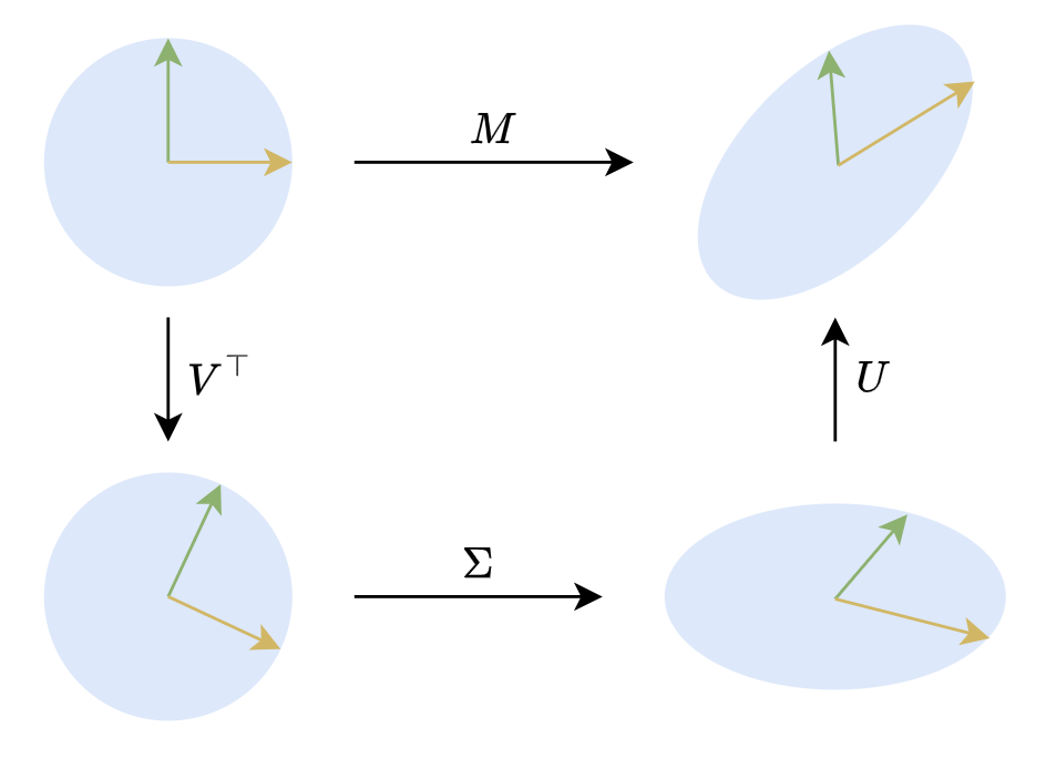
Geometric Meaning of SVD
Some Applications#
Both in theoretical analysis and numerical computation, SVD finds extremely wide application. One underlying principle is that common matrix/vector norms are invariant under orthogonal transformations. Consequently, SVD's structure—with two orthogonal matrices sandwiching a diagonal matrix—often allows conversion of many matrix-related optimization objectives into equivalent special cases involving non-negative diagonal matrices, thereby simplifying problems.
Pseudo-Inverse General Solution#
Taking the pseudo-inverse as an example, when \(\boldsymbol{A}\in\mathbb{R}^{n\times r}\) has rank \(r\), we have:
In the previous article, we derived an expression for \(\boldsymbol{A}^{\dagger}\) via differentiation, then extended it with some effort to cases where \(\boldsymbol{A}\) has rank less than \(r\). However, with SVD, the problem simplifies considerably. We can decompose \(\boldsymbol{A}\) as \(\boldsymbol{U}\boldsymbol{\Sigma} \boldsymbol{V}^{\top}\), then express \(\boldsymbol{B}\) as \(\boldsymbol{V} \boldsymbol{Z} \boldsymbol{U}^{\top}\). Note we haven't stipulated that \(\boldsymbol{Z}\) is diagonal, so \(\boldsymbol{B}=\boldsymbol{V} \boldsymbol{Z} \boldsymbol{U}^{\top}\) can always be achieved. Thus:
The last equality uses the result proved in the previous article: "orthogonal transformations preserve the Frobenius norm." Thus, we have simplified the problem to finding the pseudo-inverse of the diagonal matrix \(\boldsymbol{\Sigma}\). Next, we can express \(\boldsymbol{\Sigma} \boldsymbol{Z} - \boldsymbol{I}_n\) in block matrix form:
Here, slicing follows Python array conventions. From the final form, to minimize the Frobenius norm of \(\boldsymbol{\Sigma} \boldsymbol{Z} - \boldsymbol{I}_n\), the unique solution is \(\boldsymbol{Z}_{[:r,:r]}=\boldsymbol{\Sigma}_{[:r,:r]}^{-1}\), \(\boldsymbol{Z}_{[:r,r:]}=\boldsymbol{0}_{r\times(n-r)}\). Essentially, \(\boldsymbol{Z}\) takes the reciprocal of all non-zero elements of \(\boldsymbol{\Sigma}^{\top}\) and then transposes. We denote this as \(\boldsymbol{\Sigma}^{\dagger}\). Thus, under SVD we have:
It can be further shown that this result also applies to \(\boldsymbol{A}\) with rank less than \(r\), making it a general form. Some tutorials directly adopt this as the definition of the pseudo-inverse. Additionally, we observe that this form does not distinguish between left and right pseudo-inverses, indicating that for a given matrix, its left and right pseudo-inverses are equal. Therefore, when discussing pseudo-inverses, we need not specify left or right.
Matrix Norms#
Utilizing the result that orthogonal transformations preserve the Frobenius norm, we also obtain:
That is, the sum of squares of singular values equals the square of the Frobenius norm. Besides the Frobenius norm, SVD can also compute the "spectral norm." In the previous article, we mentioned that the Frobenius norm is just one type of matrix norm; another common matrix norm is the spectral norm induced by vector norms, defined as:
Note that the norms on the right-hand side are vector norms (length, \(2\)-norm), so this definition is well-defined. Since it is induced by the vector \(2\)-norm, it is also called the matrix \(2\)-norm. Numerically, the spectral norm of a matrix equals its largest singular value: \(\Vert \boldsymbol{M}\Vert_2 = \sigma_1\).
To prove this, simply perform SVD on \(\boldsymbol{M}\) as \(\boldsymbol{U}\boldsymbol{\Sigma} \boldsymbol{V}^{\top}\), then substitute into the spectral norm definition:
The second equality exploits the property that orthogonal matrices preserve vector norms. Now we have reduced the problem to finding the spectral norm of the diagonal matrix \(\boldsymbol{\Sigma}\), which is simpler. Let \(\boldsymbol{y} = (y_1,y_2,\cdots,y_m)\), then:
Thus \(\Vert \boldsymbol{\Sigma} \boldsymbol{y}\Vert\) does not exceed \(\sigma_1\), and equality is achieved when \(\boldsymbol{y}=(1,0,\cdots,0)\). Therefore \(\Vert \boldsymbol{M}\Vert_2=\sigma_1\). Comparing with the Frobenius norm result, we also find that \(\Vert \boldsymbol{M}\Vert_2\leq \Vert \boldsymbol{M}\Vert_F\) always holds.
Low-Rank Approximation#
Finally, we return to the main topic of this article: optimal low-rank approximation, i.e., objective (1). Decomposing \(\boldsymbol{M}\) as \(\boldsymbol{U}\boldsymbol{\Sigma} \boldsymbol{V}^{\top}\), we can write:
Note that \(\boldsymbol{U}^{\top}\boldsymbol{A}\boldsymbol{B}\boldsymbol{V}\) can still represent any matrix with rank at most \(r\). Thus, via SVD we have simplified the optimal rank-\(r\) approximation of matrix \(\boldsymbol{M}\) to the optimal rank-\(r\) approximation of the non-negative diagonal matrix \(\boldsymbol{\Sigma}\).
In "Towards Full-Parameter Fine-Tuning! The Most Exciting LoRA Improvement I've Seen (Part 1)", we used the same approach to solve a similar optimization problem:
Using SVD and the invariance of the Frobenius norm under orthogonal transformations, we obtain:
This transforms the original optimization problem for general matrix \(\boldsymbol{M}\) into a special case where \(\boldsymbol{M}\) is a non-negative diagonal matrix, reducing analysis difficulty. Note that if \(\boldsymbol{A},\boldsymbol{B}\) have rank at most \(r\), then \(\boldsymbol{A}\boldsymbol{A}^{\top}\boldsymbol{M} + \boldsymbol{M}\boldsymbol{B}^{\top}\boldsymbol{B}\) has rank at most \(2r\) (assuming \(2r < \min(n,m)\)). So the original problem also seeks an optimal rank-\(2r\) approximation of \(\boldsymbol{M}\), which after transformation to a non-negative diagonal matrix becomes the optimal rank-\(2r\) approximation of a non-negative diagonal matrix—essentially the same as the previous problem.
Theoretical Foundations#
Having affirmed the utility of SVD, we must supplement some theoretical proofs. First, we need to ensure the existence of SVD. Second, we must identify at least one computational scheme, making SVD's various applications practically feasible. Next, we will address both problems simultaneously through a unified process.
Spectral Theorem#
Before proceeding, we need to introduce the "Spectral Theorem," which can be viewed either as a special case of SVD or as its foundation:
Spectral Theorem For any real symmetric matrix \(\boldsymbol{M}\in\mathbb{R}^{n\times n}\), there exists a spectral decomposition (also called eigenvalue decomposition): \[ \boldsymbol{M} = \boldsymbol{U}\boldsymbol{\Lambda} \boldsymbol{U}^{\top} \] where \(\boldsymbol{U},\boldsymbol{\Lambda}\in\mathbb{R}^{n\times n}\), \(\boldsymbol{U}\) is an orthogonal matrix, and \(\boldsymbol{\Lambda}=\text{diag}(\lambda_1,\cdots,\lambda_n)\) is a diagonal matrix.
Essentially, the Spectral Theorem asserts that any real symmetric matrix can be diagonalized by an orthogonal matrix. This is based on the following two properties:
1. Eigenvalues and eigenvectors of real symmetric matrices are real;
2. Eigenvectors corresponding to distinct eigenvalues of a real symmetric matrix are orthogonal.
These two properties are actually simple to prove, so we won't elaborate here. Based on these, we can immediately conclude that if a real symmetric matrix \(\boldsymbol{M}\) has \(n\) distinct eigenvalues, then the Spectral Theorem holds:
Here \(\lambda_1,\lambda_2,\cdots,\lambda_n\) are eigenvalues, and \(\boldsymbol{u}_1,\boldsymbol{u}_2,\cdots,\boldsymbol{u}_n\) are corresponding unit eigen-(column)vectors. Writing in matrix multiplication form gives \(\boldsymbol{M}\boldsymbol{U}=\boldsymbol{U}\boldsymbol{\Lambda}\), so \(\boldsymbol{M} = \boldsymbol{U}\boldsymbol{\Lambda} \boldsymbol{U}^{\top}\). The difficulty in the proof lies in extending to cases with repeated eigenvalues. However, before considering a complete proof, we can gain an intuitive, albeit non-rigorous, sense that this result for distinct eigenvalues must generalize to the general case.
Why? From a numerical perspective, the probability of two real numbers being absolutely equal is almost zero, so we hardly need to consider equal eigenvalues. In more mathematical terms, real matrices with distinct eigenvalues are dense in the set of all real matrices. Therefore, we can always find a family of matrices \(\boldsymbol{M}_{\epsilon}\) such that when \(\epsilon > 0\), its eigenvalues are pairwise distinct, and when \(\epsilon \to 0\), it equals \(\boldsymbol{M}\). Consequently, each \(\boldsymbol{M}_{\epsilon}\) can be decomposed as \(\boldsymbol{U}_{\epsilon}\boldsymbol{\Lambda} _{\epsilon}\boldsymbol{U}_{\epsilon}^{\top}\). Taking \(\epsilon\to 0\) yields the spectral decomposition of \(\boldsymbol{M}\).
Mathematical Induction#
Unfortunately, the above reasoning can only serve as an intuitive but non-rigorous understanding, as transforming it into a rigorous proof remains difficult. In fact, perhaps the simplest method for rigorously proving the Spectral Theorem is mathematical induction: under the assumption that any \((n-1)\)-order real symmetric matrix can be spectrally decomposed, we prove that \(\boldsymbol{M}\) can also be spectrally decomposed.
The key idea in the proof is to decompose \(\boldsymbol{M}\) into some eigenvector and its \((n-1)\)-dimensional orthogonal subspace, allowing application of the inductive hypothesis. Specifically, let \(\lambda_1\) be a non-zero eigenvalue of \(\boldsymbol{M}\), and \(\boldsymbol{u}_1\) the corresponding unit eigenvector, so \(\boldsymbol{M}\boldsymbol{u}_1 = \lambda_1 \boldsymbol{u}_1\). We can supplement \(n-1\) unit vectors \(\boldsymbol{Q}=(\boldsymbol{q}_2,\cdots,\boldsymbol{q}_n)\) orthogonal to \(\boldsymbol{u}_1\), such that \((\boldsymbol{u}_1,\boldsymbol{q}_2,\cdots,\boldsymbol{q}_n)=(\boldsymbol{u}_1,\boldsymbol{Q})\) forms an orthogonal matrix. Now consider:
Note that \(\boldsymbol{Q}^{\top} \boldsymbol{M} \boldsymbol{Q}\) is an \((n-1)\)-order square matrix and is clearly a real symmetric matrix. By the induction hypothesis, it can be spectrally decomposed as \(\boldsymbol{V} \boldsymbol{\Lambda}_2 \boldsymbol{V}^{\top}\), where \(\boldsymbol{V}\) is an \((n-1)\)-order orthogonal matrix and \(\boldsymbol{\Lambda}_2\) is an \((n-1)\)-order diagonal matrix. Then we have \((\boldsymbol{Q}\boldsymbol{V})^{\top} \boldsymbol{M} \boldsymbol{Q}\boldsymbol{V}= \boldsymbol{\Lambda}_2\). Based on this result, consider \(\boldsymbol{U} = (\boldsymbol{u}_1, \boldsymbol{Q}\boldsymbol{V})\). It can be verified that \(\boldsymbol{U}\) is also an orthogonal matrix, and:
That is, \(\boldsymbol{U}\) is precisely the orthogonal matrix that diagonalizes \(\boldsymbol{M}\), so \(\boldsymbol{M}\) can undergo spectral decomposition. This completes the crucial step of mathematical induction.
Singular Decomposition#
At this point, all preparations are complete, and we can formally prove the existence of SVD and provide a practical computational scheme.
In the previous section, we introduced spectral decomposition. It's not difficult to notice its similarity to SVD, but there are two obvious differences: 1. Spectral decomposition applies only to real symmetric matrices, while SVD applies to any real matrix; 2. SVD's diagonal matrix \(\boldsymbol{\Sigma}\) is non-negative, but spectral decomposition's \(\boldsymbol{\Lambda}\) may not be. So what exactly is their connection? It's easy to verify that if \(\boldsymbol{M}\) has SVD \(\boldsymbol{U}\boldsymbol{\Sigma} \boldsymbol{V}^{\top}\), then:
Note that both \(\boldsymbol{\Sigma}\boldsymbol{\Sigma}^{\top}\) and \(\boldsymbol{\Sigma}^{\top}\boldsymbol{\Sigma}\) are diagonal matrices. This implies that the spectral decompositions of \(\boldsymbol{M}\boldsymbol{M}^{\top}\) and \(\boldsymbol{M}^{\top}\boldsymbol{M}\) are \(\boldsymbol{U}\boldsymbol{\Sigma}^2 \boldsymbol{U}^{\top}\) and \(\boldsymbol{V}\boldsymbol{\Sigma}^2 \boldsymbol{V}^{\top}\), respectively. This suggests that performing spectral decomposition on \(\boldsymbol{M}\boldsymbol{M}^{\top}\) and \(\boldsymbol{M}^{\top}\boldsymbol{M}\) separately might yield the SVD of \(\boldsymbol{M}\)? Indeed, this can serve as a computational approach for SVD, but we cannot directly prove that the resulting \(\boldsymbol{U},\boldsymbol{\Sigma},\boldsymbol{V}\) satisfy \(\boldsymbol{M}=\boldsymbol{U}\boldsymbol{\Sigma} \boldsymbol{V}^{\top}\).
The key to solving this is to perform spectral decomposition on only one of \(\boldsymbol{M}\boldsymbol{M}^{\top}\) or \(\boldsymbol{M}^{\top}\boldsymbol{M}\), then construct the orthogonal matrix on the other side via another method. Without loss of generality, assume \(\boldsymbol{M}\) has rank \(r \leq m\). Consider performing spectral decomposition on \(\boldsymbol{M}^{\top}\boldsymbol{M}\) as \(\boldsymbol{V}\boldsymbol{\Lambda} \boldsymbol{V}^{\top}\). Note that \(\boldsymbol{M}^{\top}\boldsymbol{M}\) is positive semidefinite, so \(\boldsymbol{\Lambda}\) is non-negative. Assume diagonal elements are already sorted in descending order; rank \(r\) implies only the first \(r\) \(\lambda_i\) are greater than 0. Define:
We can verify:
Here we adopt the convention that slicing has priority over transpose, inverse, and other matrix operations, i.e., \(\boldsymbol{U}_{[:n,:r]}^{\top}=(\boldsymbol{U}_{[:n,:r]})^{\top}\), \(\boldsymbol{\Sigma}_{[:r,:r]}^{-1}=(\boldsymbol{\Sigma}_{[:r,:r]})^{-1}\), etc. The above result shows that \(\boldsymbol{U}_{[:n,:r]}\) is part of an orthogonal matrix. Next, we have:
Note that \(\boldsymbol{M}\boldsymbol{V}\boldsymbol{V}^{\top} = \boldsymbol{M}\) always holds. \(\boldsymbol{V}_{[:m,:r]}\) comprises the first \(r\) columns of \(\boldsymbol{V}\). From \(\boldsymbol{M}^{\top}\boldsymbol{M}=\boldsymbol{V}\boldsymbol{\Lambda} \boldsymbol{V}^{\top}\), we can write \((\boldsymbol{M}\boldsymbol{V})^{\top}\boldsymbol{M}\boldsymbol{V} = \boldsymbol{\Lambda}\). Denote \(\boldsymbol{V}=(\boldsymbol{v}_1,\boldsymbol{v}_2,\cdots,\boldsymbol{v}_m)\). Then \(\Vert \boldsymbol{M}\boldsymbol{v}_i\Vert^2=\lambda_i\). Given the rank \(r\) setting, when \(i > r\), \(\lambda_i=0\), meaning \(\boldsymbol{M}\boldsymbol{v}_i\) is actually a zero vector. Thus:
This shows \(\boldsymbol{U}_{[:n,:r]}\boldsymbol{\Sigma}_{[:r,:r]}\boldsymbol{V}_{[:m,:r]}^{\top}=\boldsymbol{M}\). Combined with the fact that \(\boldsymbol{U}_{[:n,:r]}\) is part of an orthogonal matrix, we have obtained the crucial components of \(\boldsymbol{M}\)'s SVD. We only need to pad \(\boldsymbol{\Sigma}_{[:r,:r]}\) with zeros to form an \(n\times m\) matrix \(\boldsymbol{\Sigma}\), and complete \(\boldsymbol{U}_{[:n,:r]}\) to an \(n\times n\) orthogonal matrix \(\boldsymbol{U}\). Then we obtain the complete SVD form \(\boldsymbol{M}=\boldsymbol{U}\boldsymbol{\Sigma} \boldsymbol{V}^{\top}\).
Approximation Theorem#
Finally, let's not forget our ultimate goal: the optimization problem (1). With SVD, we can now present the answer:
If \(\boldsymbol{M}\in\mathbb{R}^{n\times m}\) has SVD \(\boldsymbol{U}\boldsymbol{\Sigma} \boldsymbol{V}^{\top}\), then the optimal rank-\(r\) approximation of \(\boldsymbol{M}\) is \(\boldsymbol{U}_{[:n,:r]}\boldsymbol{\Sigma}_{[:r,:r]} \boldsymbol{V}_{[:m,:r]}^{\top}\).
This is known as the Eckart-Young-Mirsky Theorem. In the "Low-Rank Approximation" section discussing SVD applications, we showed that via SVD, the optimal rank-\(r\) approximation problem for a general matrix can be reduced to the rank-\(r\) approximation of a non-negative diagonal matrix. Thus, the Eckart-Young-Mirsky Theorem essentially states that the optimal rank-\(r\) approximation of a non-negative diagonal matrix is simply the matrix retaining only the \(r\) largest diagonal elements.
Some readers might think: "Isn't this obviously true?" But the fact is, although the conclusion aligns with intuition, it is not obviously true. Let's focus on solving:
where \(\boldsymbol{A}\in\mathbb{R}^{n\times r}, \boldsymbol{B}\in\mathbb{R}^{r\times m}, \boldsymbol{\Sigma}\in\mathbb{R}^{n\times m}, r < \min(n,m)\). If \(\boldsymbol{A}\) is given, the optimal solution for \(\boldsymbol{B}\) was derived in the previous article as \(\boldsymbol{A}^{\dagger} \boldsymbol{\Sigma}\). Thus we have:
Let the SVD of matrix \(\boldsymbol{A}\) be \(\boldsymbol{U}_\boldsymbol{A}\boldsymbol{\Sigma}_\boldsymbol{A} \boldsymbol{V}_\boldsymbol{A}^{\top}\). Then \(\boldsymbol{A}^{\dagger}=\boldsymbol{V}_\boldsymbol{A} \boldsymbol{\Sigma}_\boldsymbol{A}^{\dagger} \boldsymbol{U}_\boldsymbol{A}^{\top}\), and:
From the pseudo-inverse computation formula, \(\boldsymbol{\Sigma}_\boldsymbol{A} \boldsymbol{\Sigma}_\boldsymbol{A}^{\dagger}\) is a diagonal matrix whose first \(r_\boldsymbol{A}\) diagonal elements are 1 (\(r_\boldsymbol{A}\leq r\) is the rank of \(\boldsymbol{A}\)) and the rest are 0. Thus \((\boldsymbol{\Sigma}_\boldsymbol{A} \boldsymbol{\Sigma}_\boldsymbol{A}^{\dagger} - \boldsymbol{I}_n)\boldsymbol{U}_\boldsymbol{A}^{\top}\) essentially retains only the last \(k=n-r_\boldsymbol{A}\) rows of the orthogonal matrix \(\boldsymbol{U}_\boldsymbol{A}^{\top}\). So finally we can simplify to:
Now using the Frobenius norm definition:
Note that \(0 \leq w_j \leq 1\), and \(w_1+w_2+\cdots+w_n = k\). Under these constraints, the minimum of the rightmost expression can only be the sum of the smallest \(k\) \(\sigma_j^2\) values. Since \(\sigma_j\) are already sorted in descending order:
That is, the error (squared Frobenius norm) between \(\boldsymbol{\Sigma}\) and its optimal rank-\(r\) approximation is \(\sum\limits_{j=r+1}^n \sigma_j^2\), which exactly matches the error incurred by retaining only the \(r\) largest diagonal elements. Thus we have proved that "the optimal rank-\(r\) approximation of a non-negative diagonal matrix is the matrix retaining only the \(r\) largest diagonal elements." Of course, this is just one solution; we haven't ruled out the possibility of multiple solutions.
It's worth noting that the Eckart-Young-Mirsky Theorem holds not only for the Frobenius norm but also for the spectral norm. The proof for the spectral norm is actually simpler; we won't elaborate here. Interested readers may refer to the Wikipedia entry on "Low-rank approximation".
Article Summary#
The protagonist of this article is the illustrious SVD (Singular Value Decomposition), which many readers likely already know to some extent. In this article, we primarily focused on content related to SVD and low-rank approximation, providing as straightforward proofs as possible for theoretical aspects including the existence of SVD, computation, and its connection to low-rank approximation.
Original Article: Su Jianlin. The Path to Low-Rank Approximation (Part 2): SVD. Scientific Spaces.
How to cite this translation:
BibTeX: