Weight Decay and Learning Rate from a Moving Average Perspective

Weight decay (Weight Decay) and learning rate (Learning Rate) are crucial components in LLM pre-training. Their proper configuration is one of the key factors determining the ultimate success or failure of the model. Since AdamW, the separation of Weight Decay from traditional L2 regularization has become standard practice. However, there has been limited theoretical progress on how to appropriately set Weight Decay and Learning Rate.

This article aims to introduce new insights into this problem: viewing the training process as a moving average memory of the training data and exploring how to set Weight Decay and Learning Rate to make this memory more effective.

Moving Average#

The general form of weight decay is:

where \(\boldsymbol{\theta}\) represents the parameters, \(\boldsymbol{u}\) is the update provided by the optimizer, and \(\lambda_t, \eta_t\) denote weight decay and learning rate, respectively. The sequences \(\{\lambda_t\}\) and \(\{\eta_t\}\) are referred to as the "WD Schedule" and "LR Schedule."

Introducing the notation:

For SGDM, \(\boldsymbol{u}_t=\boldsymbol{m}_t\); for RMSProp, \(\boldsymbol{u}_t= \boldsymbol{g}_t/(\sqrt{\boldsymbol{v}_t} + \epsilon)\); for Adam, \(\boldsymbol{u}_t=\hat{\boldsymbol{m}}_t\left/\left(\sqrt{\hat{\boldsymbol{v}}_t} + \epsilon\right)\right.\); for SignSGDM, \(\boldsymbol{u}_t=\text{sign}(\boldsymbol{m}_t)\); and for Muon, \(\boldsymbol{u}_t=\text{msign}(\boldsymbol{m}_t)\). Among these examples, except for SGDM, the others are adaptive learning rate optimizers.

Our starting point is the moving average (Exponential Moving Average, EMA) perspective, rewriting weight decay as:

Here, weight decay appears as a weighted average between the model parameters and \(-\boldsymbol{u}_t / \lambda_t\). The moving average perspective is not new; it has been discussed in works such as "How to set AdamW's weight decay as you scale model and dataset size" and "Power Lines: Scaling Laws for Weight Decay and Batch Size in LLM Pre-training". This article refines various aspects within this framework.

The following discussion primarily focuses on Adam, with other optimizers considered later. The calculations overlap significantly with "Asymptotic Estimation of Weight RMS in AdamW (Part 1)" and "Asymptotic Estimation of Weight RMS in AdamW (Part 2)", which readers may refer to for comparison.

Iterative Expansion#

For simplicity, assume constant \(\lambda,\eta\), and let \(\beta_3 = 1 - \lambda\eta\). Then, \(\boldsymbol{\theta}_t = \beta_3 \boldsymbol{\theta}_{t-1} + (1 - \beta_3)( -\boldsymbol{u}_t / \lambda)\). Direct iterative expansion yields:

For Adam, \(\boldsymbol{u}_t=\hat{\boldsymbol{m}}_t\left/\left(\sqrt{\hat{\boldsymbol{v}}_t} + \epsilon\right)\right.\). Typically, by the end of training, \(t\) is sufficiently large such that \(\beta_1^t,\beta_2^t\) are negligible, allowing us to ignore the distinction between \(\boldsymbol{m}_t\) and \(\hat{\boldsymbol{m}}_t\), \(\boldsymbol{v}_t\) and \(\hat{\boldsymbol{v}}_t\). Further simplifying with \(\epsilon=0\), we have \(\boldsymbol{u}_t=\boldsymbol{m}_t / \sqrt{\boldsymbol{v}_t}\). Applying the mean-field approximation:

Expanding \(\boldsymbol{m}_t,\boldsymbol{v}_t\) gives \(\boldsymbol{m}_t = (1 - \beta_1)\sum_{i=1}^t \beta_1^{t-i}\boldsymbol{g}_i\) and \(\boldsymbol{v}_t = (1 - \beta_2)\sum_{i=1}^t \beta_2^{t-i}\boldsymbol{g}_i^2\). Substituting into the above:

The summation interchange uses the identity \(\sum_{i=1}^t \sum_{j=1}^i a_i b_j = \sum_{j=1}^t \sum_{i=j}^t a_i b_j\). In summary:

The weights \(\boldsymbol{\theta}_t\), representing the training outcome, are expressed as a weighted average of \(\boldsymbol{\theta}_0\) and \(-\bar{\boldsymbol{u}}_t / \lambda\). Here, \(\boldsymbol{\theta}_0\) is the initial weight, and \(\bar{\boldsymbol{u}}_t\) is data-dependent. Under the mean-field approximation, \(\bar{\boldsymbol{u}}_t \approx \bar{\boldsymbol{m}}_t/\sqrt{\bar{\boldsymbol{v}}_t}\), with \(\bar{\boldsymbol{m}}_t\) and \(\bar{\boldsymbol{v}}_t\) being weighted sums of gradients at each step. For \(\bar{\boldsymbol{m}}_t\), the weight for gradient at step \(j\) is proportional to \(\beta_3^{t-j+1} - \beta_1^{t-j+1}\).

Memory Period#

We are primarily concerned with pre-training, which is characterized by Single-Epoch training where most data are seen only once. Thus, a key to good performance is not forgetting early data. Assuming the training data are globally shuffled, each batch can be considered equally important.

Data are linearly superimposed into \(\bar{\boldsymbol{m}}_t\) via gradients. Assuming each gradient contains only information from the current batch, a batch remains unforgotten if the coefficient \(\beta_3^{t-j+1} - \beta_1^{t-j+1}\) is not too small. Consider the function \(f(s) = \beta_3^s - \beta_1^s\), which increases then decreases. Since \(\beta_3\) is closer to 1 than \(\beta_1\), the increase is brief, and the function decays approximately exponentially at larger distances, as shown below:

Figure 1: Gradient weight as a function of distance. The coefficient decreases approximately exponentially with increasing distance from the current step.

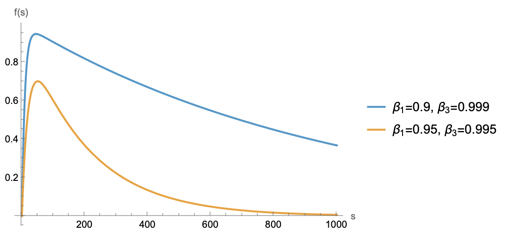
The trend shows that coefficients decrease with distance. To ensure the model remembers every batch, the coefficient at the farthest point must not be too small. Assuming a coefficient \(\geq c \in (0, 1)\) is required for memory, and for large \(s\), \(\beta_1^s \to 0\), so \(\beta_3^s - \beta_1^s\approx \beta_3^s\). Solving \(\beta_3^s\geq c\) gives \(s \leq \frac{\log c}{\log \beta_3} \approx \frac{-\log c}{\lambda\eta}\). This indicates the model can remember at most \(\mathcal{O}(1/\lambda\eta)\) steps of data, defining its memory period.

Setting \(\lambda=0\) theoretically yields an infinite memory period, eliminating forgetting concerns. However, this is not ideal. Weight decay also helps the model forget initialization. From Equation (7), the weight of initialization \(\boldsymbol{\theta}_0\) is \(\beta_3^t\). If \(\beta_3\) is too large or training steps \(t\) are too few, initialization dominates, leaving the model underfitted.

Additionally, weight decay stabilizes the model's "internal state." As derived in "Asymptotic Estimation of Weight RMS in AdamW (Part 1)", the asymptotic weight RMS for AdamW is \(\sqrt{\eta/2\lambda}\). If \(\lambda=0\), weight RMS expands at a rate of \(\eta\sqrt{t}\), potentially causing weight explosion.

Therefore, \(\beta_3\) should not be too small to avoid forgetting early data, nor too large to prevent underfitting or weight explosion. A suitable setting is to make \(1/\lambda\eta\) proportional to the number of training steps, or in multi-epoch training scenarios, proportional to the number of steps per epoch.

Dynamic Version#

In practice, dynamic LR schedules like Cosine Decay, Linear Decay, or WSD (Warmup-Stable-Decay) are more common. Thus, the static weight decay and learning rate results need extension to dynamic versions.

Starting from Equation (3) and approximating \(1 - \lambda_t \eta_t\approx e^{-\lambda_t \eta_t}\), iterative expansion yields:

where \(\kappa_t = \sum_{i=1}^t \eta_i\lambda_i\). Defining \(z_t = \sum_{i=1}^t e^{\kappa_i}\eta_i\), the same mean-field approximation holds:

Substituting expansions for \(\boldsymbol{m}_t,\boldsymbol{v}_t\):

Compared to static versions, the dynamic case retains a similar form, with gradient weights becoming more complex functions \(\bar{\beta}_1(j,t)\) and \(\bar{\beta}_2(j,t)\). For \(\beta_1,\beta_2\to 0\), they simplify to:

Optimal Scheduling#

Several analyses can follow, such as computing \(\bar{\beta}_1(j,t)\) and \(\bar{\beta}_2(j,t)\) for specific WD and LR schedules or estimating memory periods. However, we take a more ambitious approach: inversely deriving optimal WD and LR schedules.

Specifically, assuming globally shuffled data implies each batch is equally important, but static coefficients \(\bar{\beta}_1(j,t)\propto\beta_3^{t-j+1} - \beta_1^{t-j+1}\) are not constant but vary with distance, conflicting with equal importance. Ideally, they should be constant. This expectation allows solving for corresponding \(\lambda_j,\eta_j\).

For simplicity, consider the special case \(\beta_1,\beta_2\to 0\), where the equation to solve is \(e^{\kappa_j}\eta_j/z_t = c_t\), with \(c_t\) depending only on \(t\). Note that the "constant" is with respect to \(j\); \(t\) is the training endpoint, and the constant can depend on it. To simplify solving, we approximate sums with integrals, i.e., \(\kappa_s \approx \int_0^s \lambda_{\tau} \eta_{\tau} d\tau\), then the equation becomes \(\exp\left(\int_0^s \lambda_{\tau} \eta_{\tau} d\tau\right)\eta_s \approx c_t z_t\). Taking logarithms and differentiating with respect to \(s\) yields:

If \(\lambda_s\) is constant \(\lambda\), solving gives:

This is the optimal LR schedule for constant weight decay, requiring no preset endpoint \(t\) or minimum learning rate \(\eta_{\min}\), allowing infinite training similar to the stable phase of WSD while balancing gradient coefficients automatically. However, it has a drawback: as \(s\to\infty\), \(\eta_s\to 0\). From "Asymptotic Estimation of Weight RMS in AdamW (Part 2)", weight RMS tends to \(\lim\limits_{s\to\infty} \frac{\eta_s}{2\lambda_s}\), so this drawback may risk weight collapse.

To address this, consider \(\lambda_s = \alpha\eta_s\), where \(\alpha=\lambda_{\max}/\eta_{\max}\) is constant. Solving yields:

Correspondingly, \(e^{\kappa_s} \approx \sqrt{2\lambda_{\max}\eta_{\max} s + 1}, e^{\kappa_s}\eta_s \approx \eta_{\max}, z_t\approx \eta_{\max} t, \bar{\beta}_1(j,t) = \bar{\beta}_2(j,t) \approx 1/t\).

General Results#

Current results, such as Equations (13) and (14), assume \(\beta_1,\beta_2=0\). Do results change for non-zero \(\beta_1,\beta_2\)? More generally, to what extent do these results generalize to other optimizers?

First, consider \(\beta_1,\beta_2\neq 0\). When \(t\) is sufficiently large, conclusions do not change significantly. For \(\bar{\beta}_1(j,t)\), under optimal scheduling, \(e^{\kappa_i}\eta_i\) is constant (relative to \(t\)). By definition:

When \(t\) is sufficiently large, \(\beta_1^{t-j+1}\to 0\), so this can also be considered constant with respect to \(j\). As mentioned earlier, for \(\beta_1,\beta_2\), "\(t\) sufficiently large" is almost always true, so results for \(\beta_1,\beta_2=0\) can be used directly.

Regarding optimizers, previously mentioned ones (SGDM, RMSProp, Adam, SignSGDM, Muon) can be divided into two categories. SGDM is one category: its \(\bar{\boldsymbol{u}}_t\) is simply \(\bar{\boldsymbol{m}}_t\), requiring no mean-field approximation, so results up to Equation (12) apply. However, Equations (13) and (14) may not be optimal, as SGDM's asymptotic weight RMS also depends on gradient norm^reference, making analysis more complex.

The remaining optimizers (RMSProp, Adam, SignSGDM, Muon) belong to another category, all being adaptive learning rate optimizers with update rules of the homogeneous form \(\frac{\text{gradient}}{\sqrt{\text{gradient}^2}}\). In this case, if we still believe in the mean-field approximation, we obtain the same \(\bar{\boldsymbol{m}}_t\) and \(\beta_1(j,t)\), so results up to Equation (12) remain applicable. Moreover, for such homogeneous optimizers, weight RMS asymptotically scales as \(\sqrt{\eta/\lambda}\), so Equations (13) and (14) can also be reused.

Assumptions Discussion#

Our derivation is now complete. This section discusses the major assumptions underlying the derivation.

Throughout the article, two major assumptions are worth discussing. The first is the mean-field approximation, introduced in "Rethinking Learning Rate and Batch Size (Part 2): Mean Field". Mean-field approximation itself is not new—it is a classic approximation in physics—but its application to analyzing optimizer dynamics was first introduced by the author. It has been used to estimate optimizer Batch Size, Update RMS, Weight RMS, etc., with results appearing reasonable.

Regarding the effectiveness of the mean-field approximation, we cannot comment too much; it embodies a form of belief. On one hand, based on the reasonableness of existing estimates, we believe it will continue to be reasonable, at least providing valid asymptotic estimates for some scalar metrics. On the other hand, for adaptive learning rate optimizers, due to the nonlinearity of update rules, analysis difficulty increases significantly, and apart from the mean-field approximation, we have few computational tools available.

The most typical example is Muon, which involves non-element-wise operations. Previous component-wise computation methods like those used for SignSGD become ineffective, while the mean-field approximation still works (refer to "Rethinking Learning Rate and Batch Size (Part 3): Muon"). Thus, the mean-field approximation provides a unified, effective, and concise computational method for analyzing and estimating a large class of adaptive learning rate optimizers. Currently, no other method seems to achieve the same effect, so we must continue to trust it.

The second major assumption is that "each gradient contains only current batch information." This assumption is fundamentally incorrect because gradients depend not only on current batch data but also on previous parameters, which naturally contain historical information. However, we can attempt to remedy this: theoretically, each batch brings new information; otherwise, the batch would be meaningless. Thus, the remedy is to change it to "each gradient contains roughly equal incremental information."

Of course, upon careful thought, this statement is also debatable, as more learning leads to broader coverage, reducing the unique information of later batches. However, we can further argue by dividing knowledge into "patterns" and "facts." Factual knowledge—such as which mathematician discovered a particular theorem—must be memorized. Thus, we can consider changing it to "each gradient contains roughly equal factual knowledge." In practice, LR schedules derived from "treating all gradients equally" appear beneficial, so we can always attempt to construct an explanation for it.

Recent paper "How Learning Rate Decay Wastes Your Best Data in Curriculum-Based LLM Pretraining" provides indirect evidence. It considers curriculum learning with increasing data quality and finds that aggressive LR decay eliminates curriculum learning advantages. Our result shows that each batch's weight is given by Equation (11), proportional to learning rate. If LR decay is too aggressive, later high-quality data receive smaller weights, leading to suboptimal performance. Being able to explain this phenomenon conversely demonstrates the reasonableness of our assumption.

Summary#

This article interprets weight decay (WD) and learning rate (LR) from a moving average perspective and explores optimal WD and LR schedules within this framework.